Моделирование z-образного возмущения на луче Педерсена дистанционно-частотной характеристики наклонного зондирования с использованием моделей ионосферы

Ionospheric irregularities, including traveling ionospheric disturbances (TIDs), have been studied in many papers [Maeda, Handa, 1980; Ivanov et al., 1987; Boytman, Kalikhman, 1989; Vugmeyster et al., 1993; Millward et al., 1993; Hocke, Schlegel, 1996; Afraimovich et al., 2002; Ding et al., 2008]. Along with diurnal and seasonal variations of ionospheric parameters (large-scale irregularities) at ionospheric heights there are traveling ionized structures of small and medium scales.

Despite the emergence and development of space-based sensing instruments, which gave an opportunity to obtain data on the Total Electron Content [Afraimovich, Perevalova, 2006], ionospheric research with the aid of frequency-modulated continuous wave ionosondes is relevant and sometimes the only way to gain information about a communication channel. It is important to understand factors that cause distortions of distance-frequency characteristic (DFC) of oblique sounding (OS) and to deviations from mean diurnal variations in maximum observed frequencies (MOF). MOF variations with periods of more than one hour on OS paths can be attributed to large-scale TIDs passing the sounding path at F-region heights [Kutelev, Kurkin, 2011]. MOF variations with shorter periods often occur with z-shaped bends in the single-hop 1F2-mode in DFC [Vertogradov et al., 2008], which move in the course of time along the upper ray (Pedersen) from the region of higher delays to the region of lower ones (sometimes repeating this movement several times).

The purpose of this study is to model TID that causes z-shaped bends at the Pedersen ray in DFC. To simulate the propagation medium, we employ the following models: International Reference Ionosphere (IRI) with correction over real observations and the Global Model of the Ionosphere and Plasmasphere (GMIP) developed in ISTP SB RAS.

MODELING DFC

DFC of a signal is calculated using the geometrical optics approximation [Kravtsov and Orlov, 1980]. The software is implemented with the method of characteristics [Golygin et al., 2003; Mikhailov, Kurkin, 2007]. Under this approach, a path problem is solved based on numerical integration of a system of characteristic equations for a two-dimensional case, using the Runge-Kutta method of the forth order of accuracy [Bakhvalov et al., 2001]:

dr

Т = p^ ’ d т d ф 1

= " Рф, d т r dpr d т

⁵ ₊ 1„ 2 f ² д r rp ^ф ,

dp ф d т

1 1 f l ^

r I f 2 дф

⁺ P r P ф

where r , φ are polar coordinates in the plane of the radio path with respect to Earth’s center, τ is the group path (propagation time multiplied by the speed of light), f pe is the plasma frequency, f is the signal frequency, p r , p φ are components of the orienting pulse p (equal to the absolute value of refractive index n at a tangent to the trajectory in the direction of propagation). To compensate for a computational error, we make a step-by-step test to meet the eikonal equation p 2 + p ф = n ² and, if necessary, correct the orienting pulse in magnitude p .

The propagation medium is specified, taking into account results obtained in [Kiyanovsky, Sazhin, 1980], by evenly spaced vertical profiles of plasma frequency (with a step of 10 km) along the path in the great-circle arc (with a distance of ~ 80 km between nodal points). Characteristics of the propagation medium are approximated through application of second-degree two-dimensional local B-splines on a uniform grid of values [Konoplin, Orlov, 1981] for the plasma frequency and for its partial derivatives. Input parameters for calculations are taken such that the calculating time is optimal. In most cases, the integration step is 1 km. The calculation in nodes of reference values of partial derivatives is based on plasma frequency interpolation by a Lagrange polynomial:

( k - 1)!( N - k )!( - 1) i " ^{k -1} _{f (} )

( i-k )( i- 1)!( N-i )!       ’

f ( k ) = Z

⁽ k ^{- 1)!(} N ^- k ^{)!( - 1) k i} f( ₊ f ( k ) _x N     ₊ ^

( k - i )( i - 1)!( N - i )!              ’ i =r k - i   i^kt 1

i * k where k = 1, ..., N.

MODELING TID BY IRI

Ionograms often have various DFC distortions manifesting themselves as bends, loops, scattering, etc. Figure 1 shows OS ionograms with traces of TIDs obtained on two paths (Figure 2) over the observation period from March 29 to April 2, 2004.

Transmitters are located in Magadan (60° N, 150.7° E) and Khabarovsk (48.5° N, 135.1° E). A receiver is in the Tunka valley in the village of Tory (51.8° N, 103° E), at about one hundred kilometers from Irkutsk (52° N, 104° E). The length of the Khabarovsk–Tory path is ~ 2300 km; Magadan–Tory path is ~ 3030 km. The distance between the midpoints of the Khabarovsk–Tory (51.26° N, 119.57° E) and Magadan–Tory (58.2 ° N, 124.17 ° E) paths is ~ 825 km.

We can see (Figure 1) that these DFC have traces of reflections that are not characteristic of the spherically stratified ionosphere or the ionosphere with a weak horizontal gradient. The geomagnetic activity index K p in this period did not, on average, exceed 3. However, despite Earth’s magnetic field was relatively quiet those days, at certain moments there were fairly stable z-shaped or sickle-shaped bends (“sickles”) in the single-hop 1F2-mode of DFC, which moved in the course of time from the region of higher delays to the region of lower ones.

Numerical modeling with geometrical optics approximation is widely used to study TID effects on characteristics of decameter radio waves. For example, in [Balagansky, Sazhin, 2003], disturbances on OS ionograms are interpreted through numerical modeling of three-dimensional inhomogeneous wavelike TIDs for the global ionospheric model with correction. An attempt to interpret OS ionograms with z-shaped distortions at the Pedersen ray (Figure 1) was made in [Kopka, Möller, 1968], in which the authors carried out computer simulation to study effects of small horizontal variations in a layer height for a single-layer parabolic ionospheric model on 2000 and 8000 km paths. Unlike [Kopka, Möller, 1968], in this work we run simulation for conditions of the real path (Khabarovsk–Tory, the range is ~ 2300 km) over the full ionospheric profile with gradient, adapting the IRI model [Kotovich, Mikhailov, 2003].

The joint application of ionospheric models, adaptation techniques, methods for calculating propagation characteristics, and experimental data, acquired on OS paths, improves the accuracy of interpretation of observations. To adapt the IRI model, we use VS data obtained near transmission and reception points; and to acquire data at the midpoint of the path, we utilize a method of converting experimental DFC into height-frequency characteristic (VFC) [Kim et al., 2004]. The OS data conversion algorithm provides VFC for the midpoint of the path, but the ionospheric model can be corrected using only f ₀F2.

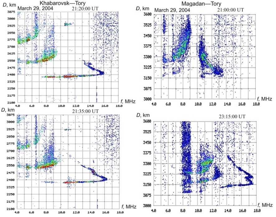
F igure 1. TIDs on OS ionogra m s obtained o v er Khabarovsk – Tory and Ma g adan–Tory pa th s

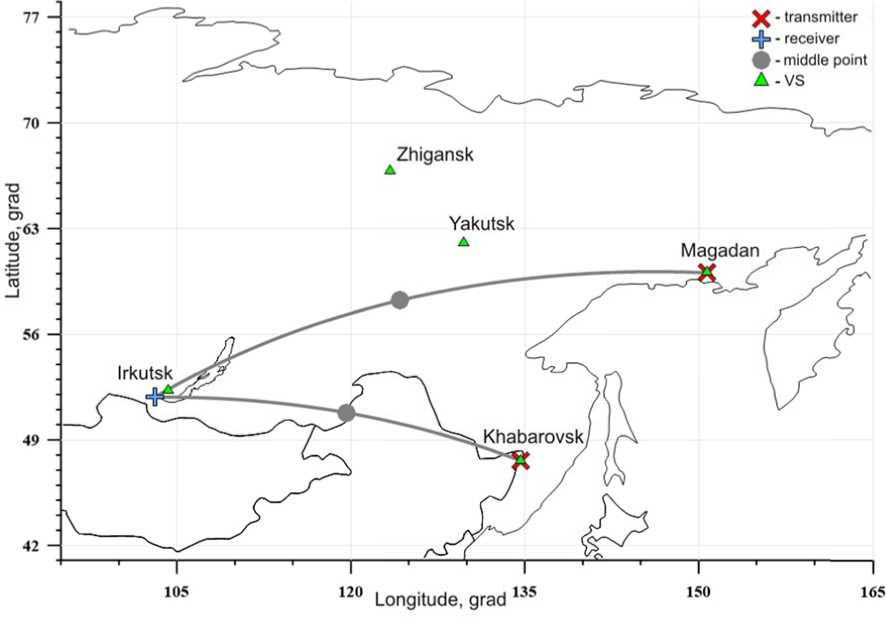
F igure 2. Map of paths

T herefore, processing of O S ionograms p rovides a set of MOF; and for the high e st point at th e upper ordin a ry ray of the 1F2-mode ( w hose path before reflectio n is close to t h e Pedersen r a y passing th e maximu m ionization height in the vicinity of the m idpoint of t h e path), freq u ency and ab s olute time o f signal propagation are also stored. Th e se data and th e modified Smith metho d [Kiyanovsk y , 1971] are u sed to compute f o F2 at the midpoint of the path by t h e algorithm described in [ K otovich et al ., 2006]. Th e n, values of the vertical electron density profile obtained with t h e IRI model are adapted f rom f _oF2 val u es acquire d at endpoints and calculat e d for the mi dp oint of the path.

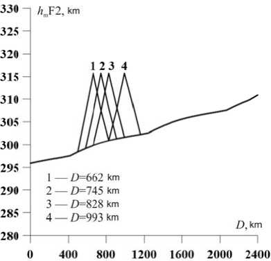
F igure 3. Disturbance model f o r h _mF2

km

О- IRI

• - IRI+

X- experiment

5 6   7 8 9 10 11 12 13 14 15 16

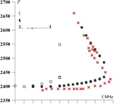
F igure 4. Estimated DFC without disturbanc e

Y et f 0 F2 values between thr e e points alon g the path are l i nearly interpo l ated.

T he propagation medium is interpolate d along the path between 2 9 nodal poi n ts given by evenly spaced vertical plasma frequenc y profiles alo n g the great-c i rcle arc.

S ince the upper ray is formed at heights n ear the F2-layer maximu m [Davies, 1965], we assu m e that the distortion at the upper ray a re caused by TIDs locate d at a close height level. A ccording to t he OS data, h m F2 ranged from 290 to 3 00 km in K h abarovsk, a n d from 300 t o 320 km in I rkutsk; therefore in 59

modeling we specify a linear va r iation in h m F 2 along the path (from a t r ansmitter to a receiver) fr o m 295 to 310 km. The increase in heig h t of the sim ul ated disturbance of the F2-layer peak e l ectron densit y at 15 km from the middle of the back g round curve corresponds t o 315 km (Figure 3). In t hi s case, we si m ulate a tria n gular-shaped disturbance w ith a base w i dth of ~ 328 k m.

I n Figure 4, unshaded circl e s indicate th e estimated D FC for Marc h 29, 21:00 U T (medium p a rameters a r e given by the IRI model, adapted fro m the averag e monthly in d ex F 10.7 = 1 11). Shaded circles show the calculated DFC after t h e adaptation of the IRI m o del from thr e e parameter s : F 10.7 (we u se the same monthly average), critical frequencies a t three point s of the path ( via linear int e rpolation al o ng the path) , and maximum heights at two (end) poi n ts of the pat h . The experi m ental DFC i s marked with crosses. After the IRI model adaptat i on has been completed, t h e deviation o f the obtain e d maximum usable frequ e ncy (MUF) from MOF observed in the e xperiment is only 2 %.

2400 е

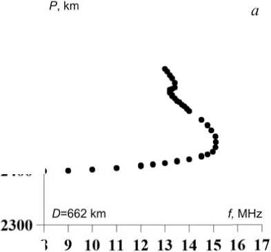
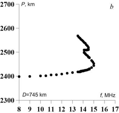
F igure 5 illustrates the sim u lated abnor m al DFC with horizontal movement of t h e h m F2 disturbance (Figure 3) along the path (from a t ransmitter to a receiver) at 6 62, 745, 828, and 993 km f ro m the trans m itter.

2700 i P, km

с

2700 P, km

2400 е

0=828 km -------------1----------------1----------------- 1----------------1----------------Г

f, MHz

8 9 10 И 12 13 14 15 16 17

2500* •

2400 .......

D=993 km/ МГц

2300 -----1-----1——।-----1-----1-----1-----11

8 9 10 11 12 13 14 15 16 17

F igure 5. Estimated DFC duri n g the h _mF2 di s turbance

ит

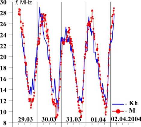
F igure 6. The diurnal variatio n of MOF for K habarovsk–To r y (Kh) and M a gadan–Tory ( M ) paths

A s the disturbance approaches the midp o int of the p a th, MUF increases (Figure 5, d ). When such a distu r bance propagates over a l a rger distance , there are no significant c h anges along the upper ra y in the estim a ted DFC.

T he correlated variability o f the diurnal M OF variatio n on two adja c ent paths (Fi g ure 2) can show the prese n ce of a moving irregularit y at h m F2. Fro m March 30 t o April 1, 2004, maxima in the diurnal v a riation of M O F of the paths under stud y were shifted in time (Fig u re 6). Knowi n g the distanc e between mi d points of the paths (~ 825 km) and their coordinates, w e qualitative l y estimated t h e velocity an d direction of irregularity. Apparently, the disturban c e was positi v e; and the M O F increase o bserved first o n the Khab a rovsk– Tory p ath and then on the Maga d an–Tory one testifies that t he irregularit y moved fro m south to nor t h. The time d elay between the disturban c e manifestati o ns suggests that its velocit y was ~ 70–1 0 0 m/s.

T he analysis of MOF aime d at determin i ng TID para m eters is desc r ibed in mor e detail in [Iv a nov et al., 2 0 06]. In addition, the lifeti m e and sizes of TIDs can be judged b y the dynami c s of “sickle” movement along the upper ray. As d educed from the experimental OS data , the duratio n of such dist o rtions ranged from 15 min to several hours. Given t y pical TID v e locities of ~ 1 00 m/s, this c orresponds t o horizontal TID dimensions of ~ 90 k m registered over ~ 1000 km. The min i mum distan c e of 90 km d e pends on th e detection interval. In fact, such irregul a rity can be l e ss than 90 k m because de f ormation of t he upper r a y during a session can be d etected only i n single DF C (rather than i n several on e s in a row).

MODELING TID BY GMIP

U nlike the semi-empirical I RI model, th e ISTP-devel o ped global m odel of the i o nosphere an d plasmasp h ere enables us to use a m i nimum set o f input data t o calculate v e rtical profile s of electron d ensity and e ffective collision frequen c y, taking int o account physical processes in Earth’ s upper atm o sphere

[Krinberg, Tashchilin, 1984; Tashchilin, Romanova, 2002; Tashchilin, Romanova, 2013]. This model is used to calculate ionospheric parameters in extreme conditions, i.e. during magnetic storms and solar flares. An important role is played here by electron density variations in the lower region of the ionosphere (E layer) during these periods as compared to the background undisturbed ionosphere because they can substantially increase signal absorption. GMIP, as other ionospheric models, retains seasonal diurnal variations in ionospheric parameters, their dependence on solar activity, season, time of day, as well as on coordinates (latitude, longitude) of radio path’s point of signal propagation, and takes into account the horizontal ionospheric irregularity at dawn and dusk hours. The complex algorithm including blocks for calculating GMIP and conditions of HF radio wave propagation allows us to compute distance-frequency and angular frequency characteristics of signals [Ponomarchuk et al., 2015].

The software package for calculating DFC enables us to represent all major propagation modes of a signal reflected from the regular ionospheric layers (E, F1, F2). Figure 7, a shows a typical DFC obtained on the Khabarovsk–Irkutsk path on March 7, 2015 at 00:36 UT. Lines depict DFC of the propagation modes 1F2, 2F2, and 3F2 calculated in the geometrical optics approximation.

Figure 7, b , c , d presents OS ionograms with traces of disturbances obtained on the Khabarovsk– Irkutsk path on March 7, 2015 at 00:56 UT, 01:06 UT, and 02:06 UT respectively. Approximately one hour after the disturbance commencement, on the ionograms there were no bends at the upper ray; and TID effects caused MOF to increase.

Internal gravity waves (IGW), which always exist in the thermosphere, play an important role in the formation of electron density irregularities in the F-region. Ionospheric effects of propagating IGW is TID, i.e. rise and subsequent fall of the F2 layer as IGW passes over the station, which usually occurs with a phase-shifted change in the electron density at the F2-layer maximum. Since the main mechanism of IGW influence on F-layer plasma is the transfer of momentum of horizontally moving neutral particles to ions, which thus acquire an additional velocity along the magnetic field, when simulating TID we specify wind momentum at a given point of the path.

To preset the propagation medium at each point of the path, we calculate the vertical profile of ionospheric parameters, using GMIP. GMIP has been developed from two models: the global semi-empirical prediction model for the D-region designed to calculate ionization in the lower ionosphere (40–100 km), and the Theoretical Model of the Ionosphere and Plasmasphere for calculating ionization at a height above 100 km.

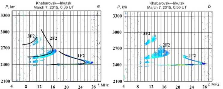
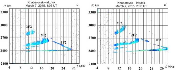
F igure 7. OS ionograms obtai n ed over the K h abarovsk–Irkutsk path on M a rch 7, 2015: 0 0 :36 UT ( a ), 0 0 :56 UT ( b ), 0 1 :06 UT ( c ), 02:06 UT ( d )

T he Theoretical Model of the Ionosph e re and Plas m asphere acc o unts for the plasma drift across geo m agnetic field lines [Krinb e rg, Tashchi l in, 1984; Tashchilin, Ro m anova, 199 5 , 2002; Tas h chilin, Rom a nova, 2013]. In the mode l , the molecu l ar ions N 2 ⁺, N O⁺, and O 2⁺ are conside r ed as the ion M⁺ of mass 30 amu with the ion density describe d as N (M⁺)= n (N 2 ⁺)+ n (N O ⁺)+ n (O 2 ⁺). T he model provides densi t ies of ions of hydrogen N (H⁺), heliu m N (He⁺), oxygen N (O⁺), m olecular io n s N (M⁺), an d electrons N _e = N (H⁺)+ N (He⁺)+ N (O⁺)+ N (M⁺), el e ctron T _e an d ion T _i tem p eratures alo n g the geomagnetic field at h ≥ 100 km from this io n ospheric reg i on to the magnetoconjugated one.

T his model is based on th e numerical s o lution of unsteady-state equations for p article balance and ther m al plasma energy in drifti n g plasma tub e s of dipole type, bases of which are at a height of 1 0 0 km. Dens i ties of all ions are calculat e d taking int o account photoionization, r ecombinatio n , and transfe r along geomagnetic field lines under t h e action of a mbipolar dif f usion and io n entrainment with the hor i zontal neutr a l wind. To calculate rates of photoion i zation of thermospheric c o mponents a n d energy spectra of primary photoelectrons, we use the reference s pectrum of solar UV radi a tion from [R i chards et al., 1994]. Electron and ion temperatures a re computed making allo w ance for the thermal con d uctivity alo n g geomagnetic field lines and the heat exchange be t ween electrons, ions, and n eutral particl e s due to elas t ic and inela s tic collisions. The heating rate of ther m al electrons i s calculated consistently b y solving the k inetic equation for photoelectron transfer in conjug a te ionospheric regions wit h respect to e n ergy losses b y photoele c trons in passing through t h e plasmasph e re.

T o describe spatio-tempor a l variations i n temperature and neutral d ensities of O , O 2 , N 2 , H, a nd N, we employ the global empirical model of the thermosphere NRLMSIS E -00 [Picone e t al., 2002] a nd determine velocities of the horizo n tal thermos p heric wind by the empiri c al models H W M07 [Drob et al., 2008] and DWM07 [Emmert et al., 2008]. T h e values of t h e integral fl u x and mean e nergy of precipitating electrons necessary to calculate auroral io n ization rates are taken in a ccordance w i th the global model of el e ctron precipitation [Hardy et al., 1987]. The electric f ield of magn e tospheric co n vection is c a lculated with the empirical model of d istribution o f magnetosph e ric convection potential at ionospheric h eights [Sojka et al., 1986].

T IDs can be driven by la r ge-scale IG W s propagati n g equatorwa r d of the au r oral heating source [Afraimovich et al., 2002]. Suc h a wave can be a momentum of the e q uatorward w i nd with its velocity depe n ding on height. In the pre s ence of the t h ermospheric wind, ions a n d electrons a re subject to a friction f o rce. Since charged particles are free to move only along the geo m agnetic field [Rishbeth, Garriott, 1969], the longitudinal friction force comp o nent (in the case of the equatorward wind) will t r ansfer charged particles up along the i n clined geom a gnetic field l ines (Figure 8 ). This mov e ment will ca u se the F2 layer to rise. The longitudin a l component U || and the v ertical comp o nent of the W wind drift dri v en by the t h ermospheric wind are calc u lated as foll o ws:

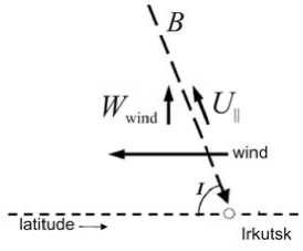
F igure 8. Thermospheric win d effect on a ch a rged compone n t

U = ( U cos D - V sin D ) co s I,

Wind = U sin I, where U and V are meridional and zonal components of the horizontal thermospheric wind, I and D are magnetic inclination and declination (for Irkutsk, I = 72.2°, D = –3.86°).

TID passage over a given point of the pa t h is modeled as strengthening of W wind :

Wwind +50 [m/s] · WTID, where WTID is a coefficient, which enables us to change the momentum. In the model calculations, we use WTID = 0.5, i.e. Wwind increased by 25 m/s. Such a momentum is specified at nodal points along the propagation path successively from a transmitter to a receiver.

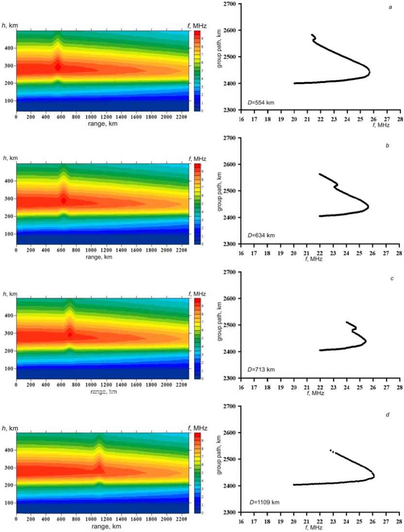
This disturbance from G M IP is model e d for the Kh a barovsk–Irk u tsk path (M a rch 7, 2015, 01:00 UT) with subsequent calculatio n of DFC in t he geometri c al optics ap p roximation. In the modeli n g, we assume that an irregularity should cover a sp a ce near the path such that reflection po i nts are in th e plane 64

of th e great-circle arc and signal paths fall i n to a receivin g point. The p aths that de v iate from the greatcircle arc are not considered.

F igure 9 shows levels of p l asma freque n cies as a function of heig h t and propa g ation path of a 23.2 MHz signal with respect to medium disturba n ces. The irregularity is sit u ated at ~ 63 4 km from th e transmitter. The propagation mediu m is specifie d by evenly spaced vertic a l electron d e nsity profile s at 30 point s along the great-circle arc. The step of calculation between adjac e nt nodal poi n ts is ~ 79 k m . The modeling reveals that in the vici n ity of the tur n ing point nearby the distu r bance, uppe r rays are foc u sed.

F igure 10 illustrates path s for the 24 M Hz signal fo r the same i nstant. At t h e given freq u ency, upper rays do not diverge. Thus, the irregul a rity has an e ffect on the g roup path o f the upper ray only when the wave disturbance is m aximal alo n g the great-circle arc from the point o f signal ent r y into the i o nosphere to the midpoint of the path ( F igure 11).

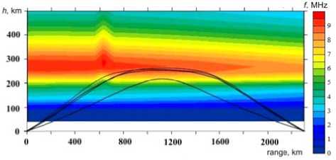
F igure 9. Paths of signal prop a gation in the d i sturbed ionosphere: f = 23.2 M Hz

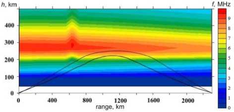
F igure 10. Paths of signal pro p agation in the d isturbed ionosphere: f = 24 M Hz

I f the maximum of irregul a rity shifts to the midpoint of the path, M UF increas e s (Figure 11, d ). If the d i sturbance is in the second half of the p a th out of the reflection p o int, there is n o TID effec t at the uppe r ray in DFC (Figure 11, e ). This is also c onfirmed by [Kopka, Möller, 1968; Gro z ov et al., 20 0 5].

T hus, the qualitative modeling has sho w n that the time displace m ent of such s ickle-shaped bends along the upper ray of the singl e -hop 1F2- m o de in DFC (Figure 11) ca n be caused b y a gust of t h e thermosp h eric wind with a speed of +25 m/s relat i ve to the bac k ground one.

■ 254И» - range, km

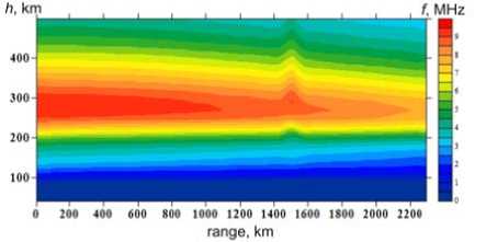
F igure 11. Simulation results for disturbance (left) and DFC (right)

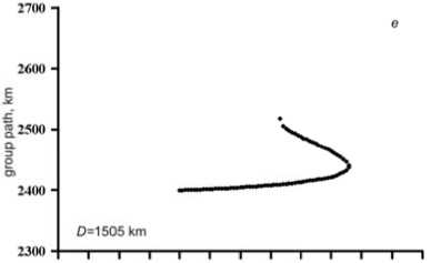
16 17 18 19 20 21 22 23 24 25 26 27 28 f, MHz

CONCLUSION

Using the ionospheric model adapted from experimental data, we have tested the disturbance model accounting for the change in h m F2in local sections of the OS path. We have shown that OS ionograms with z-shaped bends in the vicinity of the upper ray, which are not characteristic of the spherically stratified ionosphere or the ionosphere with a weak horizontal gradient, may indicate that at the moment of formation of a reflected signal, it is reflected and focused from the region of the h _mF2 local jump occurring in the first half of the path. The modeling has also revealed that with TID passing nearby the midpoint of the OS path, bends at the upper ray disappear and MOF increases. This can be used to obtain TID parameters by analyzing MOF variations from observations acquired at the network of OS paths. If the jump of h m F2 falls on the second half of the path, there is no z-shaped bend at the upper ray of the single-hop mode 1F2.

The ISTP-developed global model of the ionosphere and plasmasphere allowed us to attribute the local change in h _mF2 to the influence of the thermospheric wind differing from the background wind by 25 m/s.

The method of correcting the IRI model from experimental OS data can also be used to correct other ionospheric models capable of adapting from f 0 F2. The necessary conditions are the availability of reliable experimental OS data and the possibility of obtaining parameters of the single-hop 1F2-mode. The process of adaptation of the ionospheric model can be employed to solve the inverse problem in interpreting experimental data.

We are grateful to A.V. Tashchilin and A.V. Oinats for useful consultations.