Modelling of the time series digressions by the example of the ups of the Ural

Electric power industry is currently one of the leading sectors of the Russian economy. According to the results of electric power production in the year 2013 Russia took the third place. Almost 10% of country‘s GDP falls to the share of electric power. Equilibrium price of "Day-ahead" market (DAM) is formed in the intersection of demand and supply curves, which are acquired through the bidding auction process. Cross-picking of electric energy is being sold on the balancing market (BM), but the price formed on this market is unbeneficial to each sides of the deal. There appears a. necessity in accurate prognosing methods that give the least prognosing error.

Small scale integration is often used for forecasting of the time series that is to say predicting not the series itself or the process, but its change or accession. In this model it is offered to modify first order integration method and to use the deviations of BMI and DAM time series. This method would help to predict the possible electric power cross-pickings and, therefore, to enhance the accuracy of already existing methods of forecasting.

The offered model is based on the sample of maximum similarity of the daily digressions from DAM from the history data, of 2009 - 2014 that was acquired from an official web-site of the wholesale electric power market .

Now we get to the formal description of the model. Introduce all the necessary nomenclature: Z ( t ) = Z (1) , Z (2) ,...,Z ( T ) is a time series that represents the volume of consumed energy in the moment of time T. ZM = Z ( t ) ,..., Z ( t = M — 1) is a piece of the time series Z ( t ) , where M is the length of the sample, considering that M E { 1 , 2 , ...,T}. The length of the sample is defined as the maximum value from the stable range for prediction value of each M E [ P, ⁰ ,p ^Z t ], where P is the length of prognosis. The prognosis is built upon the model, described below. MAE (mean absolute error) is calculated through the following formula: MAE = П Y n =1 \y ( i ) — У ( i ) b ^wh^ere t is a moment of time, a datum point in the sample, moreover t E { 1 , 2 , ..., T — M + 1 }.

Modelling of the time series with the help of samples is based on the supposition that a time series is a sequence of samples [1]. Grounding on this supposition, we consider two samples of equal length and belonging to one and the same time series with difference in datum points of sequences к [2]: ZM = Z ( t ) , ...,Z ( t + M - 1) , ZMk = Z ( t - k ) ,.... Z ( t - k + M - 1) , k G { 1 , 2 , .... t - 1 }.

Consider the prognosis algorithm.

Defining of the new history sample: ZTM_{-M +1} is a sample of a time series, which values are preceding the moment of prognosis T.

Defining of the maximum similarity sample:

For each value of time delay k G { 1 , 2 , ...,T - M - 1 } the problem of approximation of the given sample ZTM_{-M +1 -k} is solved, in other words the sample is being sequentially compared to all other values of time sequence with shift to unitary vector.

Calculating the approximation through classic linear model would be improper, since the values of time series can be either positive or negative. The acquired sample is divided into 2 rows: ZT_{-M +1 -k} >  0 - for positive values of the sample and Z_{T-M +1 -k}<  0 for negative.

Then we calculate the approximate value of the sample for positive values of the sample and separately for negative using the following formula: Z_t ^M = a 1 Z_t ^M _k + а о I ^M , where a 1 and а о are coefficients. I ^M is a, unitary vector [3].

It is necessary to define the values of coefficients from the condition:

m - 1

a2 = ^ (Z(t + i)- Z (t + i))2 ^ min, t=0

in other words such that the square of deviations of model values from the real ones to is minimal [4].

Function of approximate error is given by:

M -1

S^ (a 1, а о) = ^ a2 = ^ (Z (t + i) — a 1Z (t — k + i) — a 0)2. t=0

Its value can be calculated with least-squares method [5]:

• _{7 д 7 u} . Г a 11 z IE M- ¹ Z ²( k + i ) E M-; ¹ Z ( k + i )1

Zx ' A = Z .where A = ^ 0 ] • Zx = [ EM- Z (k + i)

7_ [E£‘ Z (k + i)-Z (T - M +1+ i)]

Zr =L     EM-1 Z (T - M + 1 _i)J

On the basis of the set problem we get 2 sets of matrices A:

A ⁺=[ ^a 0 ] • A- =[ a 2 ] ■

Then the coefficients and approximate values of the sample are defined. After this the values of the correlation modulus is calculated using the formula:

M p (Z t • ZM)

E М Л z ( t + i ) - Z )( z ( t + i ) - Z )

VE£( ^m ( t + i ) - Z )² E M 1( Z ( t + i ) - Z )²

G [0 , 1] .

КРАТКИЕ СООБЩЕНИЯ

From the received values the highest possible is taken and its coherence to the time delay is found [2].

With consideration of the maximum value of time delay, coefficients and the sample length, two approximation ecpiations for positive and negative values of the sample ^ +M                             M respectively can be written: Zt = a 1 ZM k + a01M - for positive values, Zt = a3ZMk + a21M - for negative values. For the i‘esearched series the parameter M = 142.

The results of prognosis are presented on fig. 1, where History means the sample that follows the sample of maximum similarity, values of which are approximate while composing the prognosis, Forecast are predicted values, Control are real values.

The forecast error for the acquired results is 3,3%.

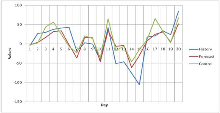
Predicting of the 20 values of BMI and DAM deviation according to maximum similarity sample using certain equations of approximation for positive and negative values

The article suggests mathematical model of forecasting the deviation of BMI and DAM according to the maximum similarity sample, using selected approximation equations for positive and negative values. The forecasting error in testing of the model was 3,3%.