Modelling the flow of character recognition results in video stream

Recently there has been a steadily growing interest in document management systems built on mobile platforms. An integral part of this kind of systems is automatic document input subsystems in which digital cameras mobile devices and web cameras act as a "scanning" device. Obvious problems [1-4], arising in the process of shooting a document made by a camera-mobile device, and subsecpiently at the stages of image processing, including the process of its recognition. Currently, these document images are of a lower quality than those obtained on the scanning device. Therefore, to obtain accurate and reliable recognition results, along with the use of traditional methods of document image recognition, it is necessary to develop new methods based on the processing of a single video stream as a digital image of the document. With this approach, there are several new problems, among which the following can be noted. The first is the problem of assessing the necessary volume of observations to make a decision on reliable recognition of a single symbol or field of the document. The second is the determination of the final estimates of the recognition results based on the integration of partial resolution of the document recognition and its fields on each frame of the video stream. To solve the integration problem, there are quite numerous nonparametric methods [1,2,5]. The most of them are based on the use of elementary statistics.

In this paper we consider the problem of construction and investigation of stochastic models describing the results of document recognition. The use of the proposed models, in our opinion, will allow us to solve the above problems productively.

We will consider the recognition of structured documents consisting of a set of text fields with pre-known properties [1,3,6]. For such fields not only tracking of sequence of recognition results of fields, but analysis of a sequence of recognition results of one symbol is possible [7].

1.    Problem Statement

Let there be a sequence of frames {I k } K ₌₁ for some document. For each I k there is a held F ( I k ). without loss of generality coiisisthig of character space A k. Че assume that character space A k is a set of n alternatees. namely {(s i ,X^k )} П ₌₁- where s i is the character code of the Cyrillic alphabet Z (s 1 =’A’, s ₂ =’Б’, etc.), X k is the probability alternative (classifier estimate) obtained at the detection of frame Ik. Introduce a notation for vectors of estimates X k = ( X k ,... ,Х П ) ^T. Let X k E T n. where T ⁿ is a simplex

n

T n = { ( X i ,...,X n ) ^T : X i >  0 ,i = 1 ,...,n ; ^ X i = 1 }.             (1)

i =1

In addition, we assume that the recognition results X k , k = 1 ,...,K, is a sample of independent equally distributed values. Let’s call the sequence { X ^k} K=1 the recognition results flow.

The paper deals with the problems of modelling (approximation) of the empirical distribution of the recognition results flow { X ^k} K ₌₁. It is possible to distinguish four stages of solving the problem [8]:

• 1)    model choice, i.e. hypothesize affiliation families of distributions;

• 2)    estimate parameters;

• 3)    evaluate quality of fit;

• 4)    estimate goodness of fit statistical tests.

2.    Preliminary Observations and Properties

In the classical formulation of the modelling problem based on the existing sample of independent random variables with unknown distribution density belonging to a certain family of parametric distributions, it is required to construct estimates of unknown parameters using the maximum likelihood principle. This problem may not have a solution if the dimension of the parameter vector is large and far exceeds the sample volume. Next, a concept is proposed that allows viewing a parametric family as a combination of distributions with vectors of smaller dimension parameters. This approach allows obtaining parameter estimates for small sample volumes of recognition results.

Here are the main symbols, as well as some definitions and results from [9]. Consider two positive random vectors X = ( X 1 ,...,X n ) and Y = ( Y 1 ,... ,Y _n ) associated with X i = Y i , where Y + = П =^₌₁ Y i. In literature the vector X is called compositional data, and the vector Y is called basis. Note that the estimates X i can be considered as an example of compositional data.

Quite often the components can be grouped according to some homogeneity criterion. In such cases, it is of interest to study the totals and relative values within each group. In order to formalize this approach, it is accepted to use amalgamation and subcomposition, which can be explained as follows. Let a ₀ = 0 < a 1 < ... < a _C- 1 < a _C = n be the set of indexes and

X i ,..., X a i \X a 1 +1 , ...,X a 2 | ... \X _a - 1 + 1 , . . . , X^                     (2)

be a complete partition (of order c — 1) of subsets оf the vector X. Based on partition (2), we define the subcomposition with index i

S , = ( X a , - 1 +1 ,-..,X a , ) X ,                            (3)

where X ⁺ = X a i - . ₁₊ i + ... + X ai, i = 1 ,... ,c . The amalgamation is the vector of the totals of the c subsets X ⁺ = ( X ⁺ ,..., X + ).

It is known [10] that for modelling of composite data the presence of the composite invariance property is essential. The basis of Y is compositionally invariant if the corresponding composition X = C ( Y ) is independent of Y ⁺. In fact, all versions of the notions of independence presented in the literature can be expressed in terms of subcompositions S i , i = 1 ,..., c , and amalgamation X ⁺. For example, consider the most popular partition case of order 1 ( c = 2). We denote in dependence by 1 and a set of independent random variables by A 1 B 1 C. Let a i = m. Then, partition independence means that S ₁ 1 S ₂ 1 X ⁺ : subcompositional in variance means that ( S ₁ , S ₂) 1 X ⁺ : neutrality on the left means that S ₁ 1 ( S ₂ ,X ⁺); neutrality on the right means that S ₂ 1 ( S ₁ , X ⁺): subcompositional hidepeiidence means that S ₁ 1 S ₂.

3.    Dirichlet Distribution and Its Generalizations

Dirichlet distribution is one of the key multidimensional distributions for composite data modelling. It plays an important role for the representation of proportions. This distribution has a simple form and has many convenient mathematical properties [П]. However, the Dirichlet distribution is considered to be insufficiently flexible. Therefore, generalizations of Dirichlet distribution were proposed by different authors [9,10].

A random vector X = (X 1 ,...,Xn)T G Tn has a Dirichlet distribution if the distribution density is as follows fD (xn; a ) = WOt] fl xa--1,                      (4)

i =1 ^{r( a} i ) i ₌₁

where a is the vector of positive parameters, a ₊ = Е П = ₁ ai.

There is a simple relation [11] between the parameters of the joint density and the marginal densities of each component X i ~ Beta ( a i ,a ₊ — a i ).

Let’s make the following transformation

X

X 1 * = X 1 , X i =--------- , i = 2 ,...,n — 1 .                  (5)

(1 — E X j ) j =1

Then for these random variables is fair nn

X * ~ Beta ( a ₁ , ^ a j ) aiid X * | X ₁ ,...,X i- ₁ ~ Beta ( a i, ^ a j ) , i = 2 ,... ,n — 1 . (6) j =2                                             j=i +1

The flexible Dirichlet distribution FDⁿ ( a, p ,t ) was first proposed in [9]. Let X = ( X ₁ ,... ,X _n ) ^T G T ⁿ. The distribution funotion of the vector X ~ FDⁿ ( a, p ,t ) is a finite mixture of Dirichlet distributions

n

FDⁿ ( x ,a, p ,t ) = ^ P i Dⁿ ( x ; a + t e i ) ,                     (7)

i =1

where ei is a vector whose elements are all equal to zero except for the г-th element which is equal to one, and the density of the distribution is as follows fFD (x; a, p,T) =

Г( a ₊ + т ) П n =i Г( a i )

Г( a i ) Г( a i + т )

where x G T n г = 1 ,...,n:a i >  0. a ₊ = n =^_{= 1} a^. 0 < p i <  1. n =^₌₁ P i = 1: т >  0.

The marginal distributions of vector X components can be represented as follows

Xi — piBeta(ai + т,a + — ai) + (1 — pi)Beta(ai, a + — ai + т), i = 1,... ,n.(9)

A vector X = ( X 1 ,..., X _n ) ^T G T ⁿ is said to follow a Connor - Mosimann distribution CM ( a, в ) if the density can be represented as follows [12]:

a = 1П^{1 Г( a} i ^{+ e} i ) ^{a   1} CTx-} i- ¹ - ( a + e i ) в п- 1 - 1

JCM(x; a, в) [    r(ai)г(в-)xi    (z ^ xj)

where x G T ⁿ; a i >  0 , i = 1 ,... ,n, в ] >  0 , j = 1 ,..., n— 1 , в о = 0. Apply a transformation similar to (5)

XГ = X1, X =----X---, i = 2,...,n — 1.(11)

(1 — E X j )

j =1

Accordingly, conditional distributions are defined as follows

X * - Beta (a 1 ,в 1)arid X* | X1 ,...,Xi-1 - Beta (ai, вi), i = 2 ,...,n — 1.(12)

The Dirichlet distribution is closely related to the parametric family of multivariate Liouville distributions. For consideration take from this family the beta-Liouville distribution. Let the vector X G (0 , 1) ⁿ have a stochastic representation X = R Y, where RL Y, R = £ ⁿ =1 Xi, R - Beta ( a,b ), Y = ( Y _L ,.. . ,Y n ) ^T G T ⁿ, Y - Dir ( a ). A random vector X is said to follow a beta-Liouville distribution. The density of beta-Liouville distribution has the form [13]:

fBL (x 1,.. .,xn; a,b,a 1,.. .a) = b-1 n

r( a )r( b ) П Г( a i ) i =1

П x^i ^-1

i =1

4.    Mathematical Model

Consider the vector X G Tn. Without loss of generality, assume that X 1 > • • • > Xn. Let's set some criteria, using whieh we can divide the composition X into two subcompositions X(1) = (X 1 ,...,Xm)T a nd X(2) = (Xm+1 ,...,Xn)T. For example, the first subcomposition includes are all elements whose values exceed a certain level L, and all the rest elements are in the second. Both subcompositions may be represented as follows

X ⁽¹⁾ = X + ¹ ) X^ , X ⁽²⁾ = X + ²⁾ X 2) ,                  (^

X +            X+ where Xj1) = Em1 Xi, Xj2) = EП= m+1 Xi, X j2) = 1 — X j1). Next, introduce new variables

Z ⁽¹⁾ =

X ⁽¹⁾

X F ^,

_Z (2) ₌

1 — X + ¹⁾⁵

R = X + .

It is possible to write an expression

X ⁽¹⁾           R ■ Z ⁽¹⁾

X⁽²⁾) = (1 — R ) ■ Z ⁽²⁾J ^,

where X⁽¹⁾ is an m -dimeiisiorial vector: X⁽²⁾ is an ( n — m )-dimeiisional vector.

Formulate assumptions for the variables included in the right part of (16).

Assumption 1. Let Z ⁽¹⁾ A Z ⁽²⁾ AR.

Assumption 2. Let R ~ Beta ( a,b ).

Assumption 3. Let Z ⁽²⁾ ~ Dir ( a ⁽²⁾).

Assumption A Let Z ⁽¹⁾ ~ Dir ( a ⁽¹⁾).

Assumption 5. Let Z ⁽¹⁾ ~ FD ( a ⁽¹⁾ , p , т ).

Assumption 6. Let Z ⁽¹⁾ ~ CM ( a ⁽¹⁾ ,в ⁽¹⁾).

For simplification of designations consider a=

_a (1)

_a (2)

= ( a 1 ,.. .,a n ) .

where a ⁽¹⁾ is an m -dimeiisioiial vector of parameters: a ⁽²⁾ is an ( n — m )-dimeiisional vector of parameters.

Using the assumptions, we construct three stochastic models for the distribution of composition X.

Model 1. If assumptions 1-4 are satisfied, the density of the composition X has the

form	f 1 ( x 1 ,.. .,X : ; a,b,a 1 ,...,a n ) = mn Г( a + b )Г E a i Г E a i i =1          i = m +1 :               X Г( а )Г( b )ПГ( a i )                                (IS) i =1

x

m xi i=1

m a- E ai-1

i =1

n xi i=m+1  /

n b— E  ai-1

i = m +1

n

П x T

- 1

Indeed, let us write density of ( Z ⁽¹⁾ , R, Z ⁽²⁾)

mn

Г(E ai) m           Г(, E ai) n rfe+b)ra- 1(i—r)b-1 x m=— n [Un-1 x :=m+1 n ।zAa-1. ив) r(a)r(b)                  п Г(ai) i=1             п Г(ai) i=m+1

i =1                       i = m +1

Now consider X 1 , . ‘ ‘ , X n , x I    The corresponding Jacobian is given by

(b      ~(b                                                (b m ⁽b ⁽ n m )

J ( z 1 , ... , z m , r , z m +1 , . . . , z n ' x 1 , . ..,x n ^,x + ) — ( ^x + ) (      ^x + )          .

Thus, from (15), (19) and (20) we have (18).

Model 2. If assumptions 1 - 3, 5 are satisfied, the density of the composition X has the form f2( x 1,.. .,Xn; a,b,a 1, ...,an,p 1,... ,Рт,т) —

m

S a i + т i =1

n

Г( a )Г( b ) П Г( a i )

m a- E ai-т -1

i =1

X

X

n

E i=mI1

x i

n b— E  ai-1

i = m + 1

n xiai-1

r( a i ) Г( a i + т )

Model 3. If assumptions 1 - 3, 6 are satisfied, the density of the composition X has the form f3 (x 1, ...,Xn; a,b,a 1 ,...,an,e 1 ,■■■, вт-1) —

n

αi i=mI1

n

r( a )r( b ) п Г( a i )

i = m I1

m

E X i=1

a- 1

n

E X i=mI1

n b— E  ai-1

i = m +1

X

m- 1

X i=1

^{Г( a} i + ^e i ) a i - 1 Г( a i )Г( e i ) ^x i

\ e i - 1 - ( a i + e i )

x j

n вт-1 -1 П a-1

xm          xi i=mI1

5.    Estimation of Model Parameters

For estimating the Dirichlet parameter vector, the principle of maximum likelihood is usually used. We assume that the parameter values that provide the maximum of the loglikelihood function are taken as estimates:

— k

k

L ⁽x n ) ; ^a ) ^— S ^log ^f D ^(x n ) ; ^a ) ^—

nn logF(£ a,) -£ i=1         i=1

j =1

n log r(ai) + E (ai - 1) log Gi i=1

,

n ₁

where G i — (П x ji ) k , i — 1 ,... ,n.

j =1

It is known [14] that the function L is globally concave, since the Dirichlet distribution belongs to the exponential family, and the Newton - Raphson algorithm converges to the global optimum [11,15].

Estimation of the parameters of a flexible Dirichlet distribution is considered as the problem of separating a finite mixture of Dirichlet distributions, for the solution of which the EM algorithm [16, 17] can be suitably adapted. Suppose we have k independent observations xj, j = 1,..., k, each having a distribution (8). Further complete vector data xc is given by:

x c = ( x , v ) = ( x i , v i ,..., x k , v k ) , (24)

where vector v j = ( V j 1 ,... ,V jn ) represents the nlissing data, with V ji being equal to 1 if the j -th observation has arisen from the f -th component of the mixture model and 0 otherwise.

The log-likelihood function with respect to (7) and (24) has the form kn log Lc (0) = EEVji [log Pi + log fD (xj; a + тei)],                (25)

j=i i=i where 0 = (a, p,т); fD(xj; a + тei) is the Dirichlet density.

The s + 1 step of the EM algorithm can be described as follows.

E-step: given the current parameter estimates 0(s) = (a(s), p(s), т(s)) andx= (x1,..., xk), calculate the conditional expectation of the complete-data log-likelihood kn

Q ( 0 ; 0 ^{( s} ) ) = EE P i ( x j ; 0 ⁽ s ) )[log P i + log f D ( x j ; a + т e i )] ,            (26)

j=i i=i where pi(xj; 0(s)) represents "posternor" probability that xj belongs to the f-th component of the mixture given 0(s) which is defined as follows

P i ^(x j ; ⁰ ) =

P i f D ( x j ; a + т e i ) E n =i P r ^f D ^(x j ; ^{a + т e} r )

f = 1 ,.

n.

M-step: maximize (26) to obtain the maximum likelihood estimates of 0 ^{( s +1)}

0 ⁽ s +1) = _arg_max Q ( 0 ; 0 ^{( s} ) ) . θ

In particular, we have p ^{( s +1)} = k E k =1 P i (x j ; 0 ^{( s} ) ) , f = 1 ,... ,n — 1, whereas a ^{( s +1)} ,т ^{( s +1)} can be computed by implementing a Newton - Raphson method. Iterating occurs until the "sufficiently small" change of the observed log-likelihood (or the parameter estimates) is reached.

Estimates of the parameters of the Connor - Mosimann distribution can be obtained using properties (12) [12]. Perform the estimation of the parameters of the beta distribution, a _r , в _г ( r = 1 ,...,n — 1), and take the resulting estimates for estimates of the prior distribution.

6.    Applying Criteria to Rank a Model

In this section, we consider the problem of selection a model from a set of competing models, which gives the best in the sense of not approaching the characteristic of the studied flow of recognition results. In modern statistics analysis for the purposes of ranking models uses a simple and effective tool - the Akaike information criterion (AIC), which can be represented as follows

n

Q aic ( F ^{( k} ) ,0 ^{( k} ) ) = — 2 ^ In f ^{( k} ) ( y j ; 0 ^{( k} ) ) + 2 q ^{( k} ) ,                   (29)

j=i where F(k) is the fc-th model: f(k)(•) is the distribution density for F(k): yj is the observation, j = 1 ,...,n; в(k) is the vector-parameter for F(k): q(k) is the number of parameters on which F(k) depends.

The choice of the model consists in ranking the models in accordance with the values of the Q AIC and the preference of the model with its lowest value.

Remark 1. Based on the AIC, we can construct a partition rule for the composition X. Suppose that for some set of (limeiisions of subcompositfoiis M = {m _min ,... ,m _max }. assumptions 1-3 hold. Then the recpiired dimension for, for example, model 1 can be defined as the solution of the problem

K

m * = arg min ( — 2 5 In f ( X X k ,...,Х П ; a,b,a 1 ,...,a _m , 1 ,..., 1) + 2 m ) .     (30)

meM k=(

It is easy to see that the obtained results (18), (21), and (22) differ in the type of distribution that describes the value of Хщ. Therefore, we confine ourselves to calculating the values of the partial criterion Q AIC (Table 1).

Table 1

Models	Q AIC
Model 1 (Dirichlet distribution)	— 221,73
Model 2 ( flexible Dirichlet distribution)	— 228,50
Model 3 (Connor - Mosimann distribution)	— 234,39

7.    Test of Models Fit

In this section, we consider the cpiestion of how well the proposed models are consistent with the observations. Before proceeding to the construction of objective quantitative estimates, it is useful to subject the obtained models to the procedure of informal graphic diagnostics, that is, to compare the sample data with the parametric model by graphic methods. To visualize the quality-of-fit of models, we use the so-called "Q-Q (quantilequantile) plot", which is a method for comparing the empirical and the theoretical distributions by plotting their quantiles against each other. If the theoretical distribution is well matched, the points on the plot are located along a straight line. Figs. 1 to 4 show the graphs for the proposed models.

Before proceeding to the formulation and testing of the hypotheses of interest, we give the formula of "standardization" X — Beta ( a,b )

X

^X • = I ( ^X ; a,b )= B ⁽ X j “’b ¹ =^Tr f -- ⁽(1 — t ) b ^{- (} dt,          (31)

B ( a, b )       B ( a, b )

where I ( z,a,b ) is the regularized inccmiplete beta, function; B ( z,a,b ) is the incomplete beta function; B ( a,b ) is the beta function. It is known [18] that the transformed random variable has the following property

X * - Beta (1 , 1) .                                  (32)

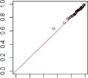
0.0 0.2 0.4 0.6 0.8 1.0

Fig. 1. The Q-Q plot for the variable X +1) in the verification of assumption 2

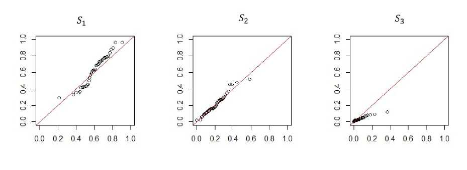
Fig. 2. The Q-Q plot for the variable X ⁽¹⁾ in model 1

We need a similar to (31) transformation formula for Y corresponding to a mixture of beta distributions

Y — p • Beta ( a 1 , a ₂) + (1 — p ) • Beta ( b 1 ,b ₂) .                     (33)

Introduce a transformation

Y * = p • I ( Y ; a 1 , a 2) + (1 — p ) • I ( Y ; b 1 , b 2) ,                        (34)

then Y * - Beta (1 , 1).

Formally, all hypotheses of goodness-of-fit necessary for our purposes have a general form. Let X 1 ,..., X n be a sequence of independent identically distributed random variables with distribution F. Then the null hypothesis is

H о : F ( x ) = I ( x ;1 , 1) .

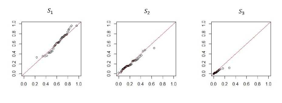
Fig. 3. The Q-Q plot for Hie variable X⁽¹⁾ in model 2

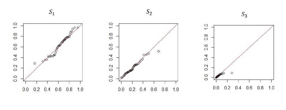
Fig. 4. The Q-Q plot for the variable X⁽¹⁾ in model 3

To verify the correspondence between the sample distribution and the theoretical law, we use the Anderson-Darling tests of goodness-of-fit [19], based on statistic [20]

n

Sq = -n - 2£ i=1

i ^ i— T ‘n F ⁽ x^ H¹

2 i

-

-

2 n

1J ln(1 - F ( X i ,0 )) j -

We point out that large values of S _Q statistics indicate poor compliance. The distribution of the statistics S Q rapidly approaches the asymptotic distribution, which has the form [21]

a 2( S ) =

2П^ 'A, ,„r( j + 1 )(4j + 1) f (4j + 1)2 n2 — g —1)j Г(2)Г(j + 1) exp [--— v 1   { s (4j + 1)2 *2 y2 L

^XJ ^Ъ -1 -   8 S ---T y ^-

X

For practical purposes, this distribution may be used provided that the sample size is greater than 5 [19].

In conclusion, consider the hypothesis testing scheme. We take assumption 4. Since Z ⁽¹⁾ ~ Dir ( a ⁽¹⁾), using properties (5) and (6) of the Dirichlet distribution, one can obtain

Z * = Z J ¹ ) ,

Z i ^∗

ZZ

(1 - E 1 z j¹) j =1

Z * — Beta ( a 11) , £ a j 1) ) , j =2

m

Z * Z ⁽¹⁾ ,...,Z - - Beta ( a ⁽¹⁾ , £ a j 1) ) , i = 2 ,...,m - 1 . j = i +1

Apply the transformation (31) to Z * and obtain

Y1 = I (Z *; a 11’, £ aj У, m        j=2

Y i = ^{1 (} Z * ; ^{a (1)} , ^{£ a} j ^x)) ,i = 1 ,...,m - ¹ . j = i +1

Then, given (32), we can formulate the hypothesis of goodness-of-fit in the following form

H о : F i ( y ) = I ( y ;1 , 1) ,                                   (40)

where F i ( y ) is the distribution function of Y i , i = 1 ,... ,m — 1: I ( y, 1 , 1) is the regularized incomplete beta function with parameters (1,1).

Table 2

The results of the goodness-of-fit test

Alternative	Model	S Q	p -value
	1	1,4679	0,1844
	2	0,67315	0,5807
	3	0,51872	0,7273
	1	1,0981	0,3095
	2	0,51691	0,7286
	3	0,13964	0,9992

As it can be seen, when setting the significance level a <  0 , 18, there is no cause for rejecting the hypotheses tested by the goodness-of-fit test for all models.

Conclusion

In this paper we propose new probabilistic models describing the results of document recognition in video stream. The concept of the flow of recognition results is introduced. The considered models suggest that the result of sign recognition in the field of the document can be represented as a combination of random variables and random vectors. For various assumptions, expressions for the density of the results of sign recognition are obtained. Methods for parameters estimation are presented. The Akaike information criterion is used for ranking models. Tests that confirmed the adequacy of the stochastic models were carried out. In conclusion, note that the solution of the problem of integration the parameters obtained by simulation of the flow of the recognition results can be used for [7].

Acknowledgement. This work is supported by Russian Foundation for Basic Research (projects No. 16-07-01051 and 17-29-03297).