Multi-Objective Optimal Dispatch Solution of Solar-Wind-Thermal System Using Improved Stochastic Fractal Search Algorithm

Author: Tushar Tyagi, Hari Mohan Dubey, Manjaree Pandit
Journal: International Journal of Information Technology and Computer Science(IJITCS) @ijitcs
Article in issue: 11 Vol. 8, 2016.
Free access
This paper presents solution of multi-objective optimal dispatch (MOOD) problem of solar-wind-thermal system by improved stochastic fractal search (ISFSA) algorithm. Stochastic fractal search (SFSA) is inspired by the phenomenon of natural growth called fractal. It utilizes the concept of creating fractals for conducting a search through the problem domain with the help of two main operations diffusion and updating. To improve the exploration and exploitation capability of SFSA, scale factor is used in place of random operator. The SFSA and proposed ISFSA is implemented and tested on six different multi objective complex test systems of power system. TOPSIS is used here as a decision making tool to find the best compromise solution between the two conflicting objectives. The outcomes of simulation results are also compared with recent reported methods to confirm the superiority and validation of proposed approach.
Meta-heuristic, MOOD, TOPSIS, Fractals, Renewable energy
Short address: https://sciup.org/15012590
IDR: 15012590
Text of the scientific article Multi-Objective Optimal Dispatch Solution of Solar-Wind-Thermal System Using Improved Stochastic Fractal Search Algorithm
Published Online November 2016 in MECS DOI: 10.5815/ijitcs.2016.11.08
Economic load dispatch (ELD) is an important issue related to power system operation and control with goal is to reduce the total operating cost of electricity generation while satisfying all complex practical operating constraints. With the increase of environment awareness, pollution contributed by the thermal power plants, the ELD cannot fulfill the sustainability of the environment because of high amount of emitted pollutants. A possible solution of this problem is to switch to the low emission fuels but this is economical in long term due to its high price and low availability. On the other hand, economic emission dispatch (EED) recently becoming more popular. In EED both cost and emission minimized together for the optimal operation of the thermal power plant and sustainability of the environment without switching to low emission fuels.
EED is a complicated multi-objective constrained optimization problem with two competing objectives as cost and emission. These problems are solved by converting the problem as single objective problem using weighted sum approach. Different weights are assigned to fuel cost and emission to get an optimal Pareto front, which helps to find out the best compromise solution (BCS).
Earlier EED was solved by goal programming method [1] or weighted min-max method [2]. But in the last decade various nature inspired algorithm were developed to solve the EED problem like Differential Evolution (DE) [3], simulated annealing (SA) algorithm [4], Bacterial foraging algorithm (BFA) [5]- [6] Teaching learning based optimization (TLBO) [7], gravitational search algorithm(GSA) [8], Real coded Chemical Reaction algorithm(RCCRO) [9], Backtracking search algorithm (BSA) [10] and etc. Also algorithm likeCuckoo Search Algorithm (CSA) [25],Cat Swarm Optimization (CSO)[26] and Ant Colony Optimization(ACO) [27] are used for optimization of real world problem.
Demand of electricity is increasing day by day and hence utilization of renewable energy resources such as wind and solar power has been increasing over the past decade to reduce the energy crisis as well as to reduce environmental pollution especially global warming.
However large scale integration of wind and solar power into existing power grid creates new operational challenges in the resulting ELD problem. The main problem associated with photo-voltaic (PV) system is weather controlled power generation and very high initial capital cost as compared to the same size of a diesel generator but the operating cost is very low and also the pollution is zero for the PV system. On the other hand, unpredictable nature of wind power creates more complication in ELD model. Hence reformulation of classical ELD model [11] is required considering issues as probabilistic based modeling of wind power, Impact of solar and wind power on emission emitted by thermal power plant. Also complex model of combined solarwind-thermal system requires efficient algorithm. The wind integrated ED modeling can be presented in [12-14]. Modeling of hybrid solar-wind system is presented in [15] whereas modeling of integrated solar-wind-thermal system is presented in [16]. A comprehensive review of hybrid renewable energy system by evolutionary algorithms is presented in [17].
In this paper a novel optimization algorithm namely Improved Stochastic Fractal Search Algorithm (ISFSA) is used to solve the MOOD problems with and withoutrenewable power integration. ISFSA utilizes scale factor in place of random operator in Stochastic Fractal Search Algorithm (SFSA) [18] to enhance exploration and exploitation capability during optimization.
This paper is organized as: Problem formulation for MOOD problem, modeling of PV system and modeling of wind farm are presented in section 2. The idea behind SFSA and its improvisation is presented in section 3 and section 4. TOPSIS for selection of best compromise solution is presented in section 5. The implementation process of ISFSA for solution of MOOD problem are depicted in section 6, whereas section 7 presents result and discussion of simulation results. Finally concluding remarks is presented in section 8.
-
II. Multi Objective Optimal Dispatch
The objective for a solar-wind-thermal system is the simultaneous minimization of total operating cost and emitted emission.
-
A. Minimization of Cost:
As the solar power plant has no operating cost, Total operating cost (Ft) consist thermal cost and the cost associated with wind power depicted as:
min F t v ;- /.' ,, (;. ).v ; /. ' (P -j .) (1)
Ftk(Pl) is thermal cost and Fw(P^lTld) is the cost associated with wind power generation. The cost associated with thermal power generation can be represented as:
F tn (Pd = № + b i P i + с * )($/Ьг.) (2)
Where a i, b i, and c i are the fuel cost coefficients of ith thermal unit.
Considering valve point loading (VPL) effect thermal power generation cost depicted as:
F tn( Pi) = « i P2 + btPt + c * + Id i SinQe^P™ - P i ))|($/hr.)
Where, d i and e i are fuel cost coefficients corresponding to VPL effect; m is the number of thermal units.
The cost associated with wind power output using wind power coefficient K j as given hereunder [12]
Fw(P2i„d) = Z"=i^;XP2i„d(4)
n is the number of wind farm.
-
B. Minimization of Emission:
Here objective is to minimize emission depicted as:
min Et = T™iEth(Pd(5)
Etn(Pd = («tP?+№+Yt)(6)
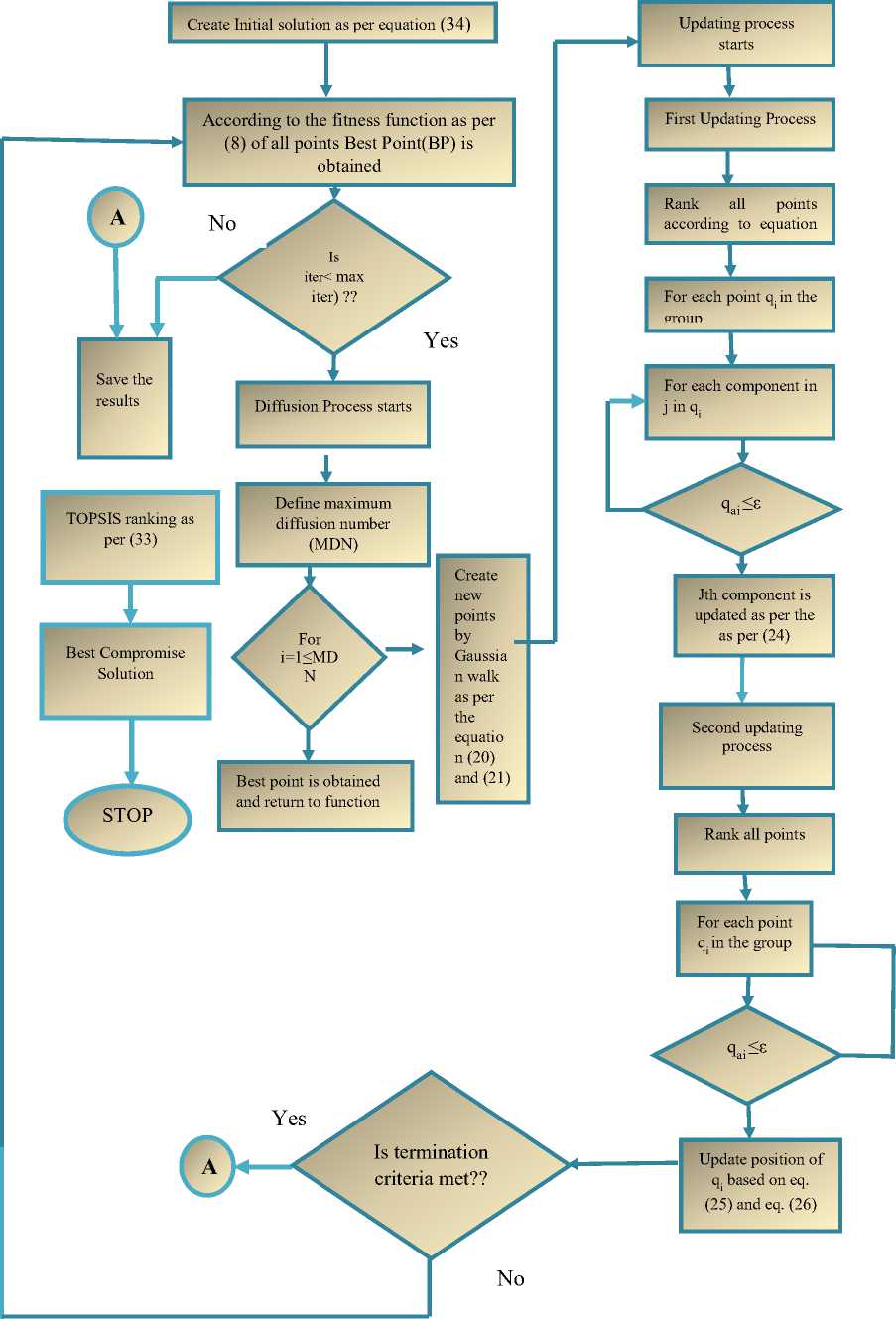
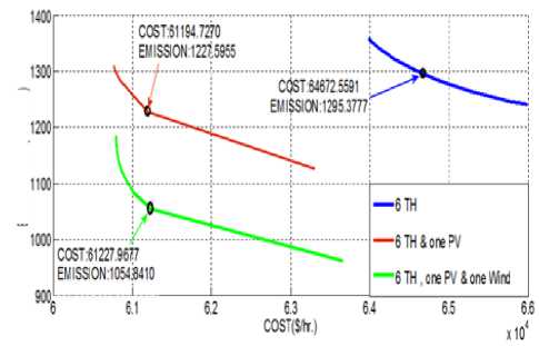
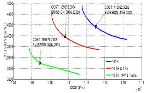
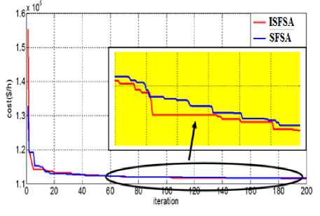
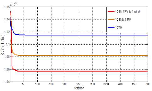
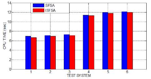
Etn(Pi) = (aiP? +/?iPi+Yi) + Eth is the total amount of emission in ton/hr, andai,Pi,A* , i^, a* are the emission coefficients of ith generator. C. Problem formulation of MOOD Here bi-objective problem is converted into a single objective one using weighted sum approach as [22]: Ftotal = w xFt + (1 -w)xEt; w E (0,1)(8) Subjected to following constraints D. Equality constraints PD +Pl = TU Pi +Ppv +T}=iPjind(9) PD represents the system power demand (MW), PL is the total transmission loss of the system (MW). PL is obtained using B-matrix coefficient as [11]: Pl^i Tj^i PiBPXP; BOiPi+Boo E. Inequality constraints Generation power should lie within minimum and maximum values. P^n^P, Pimin and Pimax is the minimum and maximum generation capacity for ith thermal units. II -A. Modeling of Photo-Voltaic System Power output of photo-voltaic (PV) system is represented as [20]: ppv = pAA (12) Where Ppv is the power output in MW/h, A is the total area of the photo-voltaic cell in m2, Я (KWh/m2) is the total radiation incident on PV system and p is the system efficiency. P = PiP2Pf (13) Where, pi is the module efficiency, p2 is the power conditioning efficiency and P^ is the packing factor. Pi = pr[1-P(TC-Tref)] (14) Where, pr is the module reference efficiency, P is array efficiency temperature coefficient, Tcis the monthly average cell temperature and TTej is the reference temperature. The radiation and temperature data are adopted from [21], and also presented in Appendix A. II-B. Modeling of Wind Farm Exact wind speed and power forecast majorly affects wind farm ideal dispatch. The wind velocity is an arbitrary variable and wind power imparts a nonlinear connection to it. The wind speed information from different places is found to take after Weibull distribution nearly and it is use for processing wind speed and wind power. Probability density function of wind velocity is expressed as [12]: pdf (и) = 1exp[-б/] (15) Hera α and β are shape and scale factor respectively. The wind power (W) can be represented as a stochastic variable and calculated from wind speed as [12]. PJ' wind. ( 0 I P iR J rwind t^in^Wind V Иу—И^ (и< uCi or и > Uco) ( итco ) (16) ( Uci < U < Ut ) Here ит, Uci and Uco are rated wind speed, cut-in speed and cut-out speed respectively. P2ind is the wind power output of jth wind unit. It is quite clear from (16) that when wind speed is either less than the cut-in speed or greater than the cut-out speed the wind power output is zero. The power output of the wind unit is a continuous variable when the wind speed is between the rated and cut-in speed and the pdf is given as per the (15) The total of all wind generator yields is taken as one random variable P.j,iml and the pdf is given by pdf(Pwind) = 13-1 ( ЗУИп P jR a pwinda l+^V • ^wind ' a . exp (©—!)• Here у = To describe the condition that the available power is not ample to satisfy the total demand with losses, a probabilistic tolerance 6a is chosen to model the uncertainty of wind power availability. In context to this the power balance constraint in (9) with wind and solar power is modified as expressed below. PT(Xl=iPWind + ^™!pi + Ppv< (Pd + PLoss)< 5a(18) A smaller value of 6a decreases the risk of not enough wind power and increases the thermal generation to ensure the good reserve capacity. III. Stocastic Fractal Search Algorithm (SFSA) Stochastic fractal search is a bio inspired algorithm developed by Hamid Salimi in 2015 [18]. It is a metaheuristic type algorithm which imitates the phenomenon of natural growth. It used the mathematical tool of fractal to imitate the growth. A fractal is a repeated graphical pattern which can be observed on many natural objects like leaves of trees, wings of peacock or patterns created in the sky due to electrical discharge. The SFSA utilizes the concept of creating fractals for conducting a search through the problem domain. The random fractals are generated by using any mathematical method like Levy flight, Gaussian walks, percolation clusters or Brownian motion. The main operations performed are diffusion and updating. In SFSA diffusion is carried out using Gaussian distribution. Each solution diffuses around its current position and generates similar solutions until a cluster is formed, promoting exploitation by each point around its current position. Updating is done in two steps to change the position of each solution. The first step mutates the elements of solution points and in the second step the whole solution is changed. Updating process is carried out on the basis of a probability assigned to each solution such that better solutions have lesser probability of change and higher chances of being retained unaltered. IV. Improved Stocastic Fractal Search Algorithm (ISFSA) The initial solutions are generated according to the equation depicted below within specified upper limit (UB) and lower limit (LB) rt = LB + F * (UB — LB) (19) where F is the user defined parameter. Stochastic Fractal Search has two important processes called diffusion and updating which are discussed as below. A. Diffusion Process Here points are generated in the search space to enhance exploitation capability of an algorithm that increases the probability of finding local minima. To generate different points Gaussian walks is utilized as per the (20) and (21). GW1 = gaussian(pBP, a) + e x BP — s' x rt (20) GW2 = gaussian(pq,o) (21) Where ε and ἐ are uniformly distributed random numbers between 0 and 1, r and BP arei£hpoint and best point in the group respectively. gBP = |BP| and gq = |г,|, о log^ x (r, - BP) The factor log^ decreases the size of the Gaussian g jumps as iteration(g) growths during simulation. B. Updating Process After initialization as in (19) all points in the search space, their fitness is evaluated and the best point (BP) is identified, then this point is diffused around the initial position and different points are generated by (20) or Eq. (21). Then ranking process is carried out for all points based on their fitness. On the basis of fitness of points probabilities are assigned to all these points uniformly to these points according to the (23). ral rank(ri) N Where, rank(rl)is the r ank of point r, among the other points in the group and N is the number of points in the group. For each point r, in group based on either condition ra, < e is satisfied or not, the jthcomponent of r,is updated according to the equation below otherwise it remains unchanged. r’ = r (j)-e x (rt(j) - г,(])) (24) rt is the new modified position of r, , rr and rt are random selected points. In second updating phase, the positions of all points are modified with respect to the position of other points in the group. It helps to improve the quality of exploration. All points obtained from the first updating process are ranked again according to the (23) If ra, < e for the imposition is held for a new pointr,' , the current position of rt i’ is modified according to the (25) and (26) as depicted below otherwise remains unchanged. r' = r' + s' x (rt - BP) if s'< 0.5 (25) r” = r/ + s' x (rt - (rr') if s’ > 0.5 (26) Where rt and rr' are random selected points obtained from the first updating process, s' is random number generated by the Gaussian distribution. If the fitness of new solution is found to be better, then only rf is replaced by rt. V. Topsis TOPSIS stands for technique for order preference by similarity to an ideal solution (TOPSIS) [23]. TOPSIS is a tool to find the best compromise solution between the conflicting objectives. TOPSIS tries to find the solution which is nearer to the ideal solution. Working of TOPSIS is summed up here-under in steps [24]. Step-1 In step-1 the normalized decision matrix is obtained as mentioned below: b,j a,j = — — f or i = 1,2, —--k; j = 1,2, — — I 15ггт(Ьц) Where, a,j and b^ are normalized and original decision matrix and k is the number of alternative solution and l is the number of alternatives. Step-2 In step-2 normalized weighted matrix is calculated from the normalized decision matrix as mentioned in step-1, which is calculated from (28) elj = Wj x a,j (28) Wj is a matrix in which weights are assigned to the objectives and e,j is the weighted normalized decision matrix. Step-3 In step-3 positive and negative ideal solution are identified as per(29) and (30) respectively. p* = [ei,e2,---e*] and 6* = {max(e,j) if jej; min(0y) if jej'} (29) P' = [e1, e2,---en] and e; = {min(e,j) if jej; max(e,j) if jej'} (30) Step-4 In step-4 geometric distances from the positive and negative ideal solutions are calculated as per the (31) and (32) Ц* = ^£j=1(6tj - e;)2)(31) H’ = ^Ёйсё,"-"ё'у(32) Step-5 In this step TOPSIS rank is calculated with respect to the closeness of ideal solution as: ‘ 0,=^ Higher values of TOPSIS rank indicates that the equivalent solution is close to the ideal solution. Fig.1. Implentation of flow chart of ISFSA in MOOD problem VI. Implementation of ISFSA for Solution of Multi Objective Optimal Dispatch In this section implementation of ISFSA is explained for economic emission dispatch problem. The step wise solution is given below. Step-1 In this step all the random solution (Points) are evaluated as per the (34). Pomts=P™" + Fx (P™M - P™") (34) WhereP™'" and P™n are the maximum and minimum power limits of Ith generator and F is scale factor. Step-2 Fitness of points generated in step-1 is calculated as per the (8) by satisfying all the operating constraints given by (9), (11) and(16). After ranking by (23) best points are evaluated according to their fitness. The TOPSIS ranking is done as per (33) to get best compromise solution(BCS). For TOPSIS ranking single objective function is considered alone to minimized among the multi-objective function by assigning weight factor for that particular as 1 and for other objective remains zero. On the other hand, if all objective function among ‘x’ objectives required to be minimizes at a time, the weight assigned to each objective is considered as 1/x. Step-3 The best points obtained as in step 2 are diffused around its neighbouring position to generate other points in the search space as per (20) and (21). Step-4 Fitness of diffused points of step-3 are evaluated again by (8) and has to satisfy operating constraints depicted in (9), (11) and(16) and re-ranking has been done. Step-5 updating process is carried out by(24). They are ranked again as in step-2, till the termination criterion has not been met, If the termination criterion is not met then from step-1 to step-5 are repeated again. Whole solution procedure is depicted using flowchart in “Fig. 1”. VII. Result and Discussion In order to validate the potential ISFSA is applied to six different standard test systems. These optimization approaches are implemented using MATLAB R2009a and the system configuration is Intel core i5 processor with 2.20 GHz and 4 GB RAM. A. Desescription Of Test Systems 1) Test system-1 It consists of six thermal generating units [7]. The fuel cost and emission function is convex in nature. Transmission losses are also taken into the account. The system demand is 1200 MW. 2) Test system -2 Here a solar plant with maximum power output of 50 MW and six thermal units are considered for analysis. Fuel cost, emission transmission loss and power demand are set as in test system 1. 3) Test system -3 In this test system having six thermal units, one solar power plant and one wind farm. The cost coefficient for wind farm considered as kr =1, kp=5, rated power output (P„tnd) as 120 MW. The other constants are uci=5, uco=45 and ur=15. The shape and scale factor as 1 and 15 respectively. Fuel cost, emission, transmission loss and power demand are set similar to test system 1. 4) Test system -4 This test system has ten thermal units with valve point loading (VPL) effects. The entire Fuel cost, emission and B-loss coefficients data were adopted from [8]. Power Demand for this is 2000 MW. 5) Test system -5 In this test system there are ten thermal units with one solar power plant. Fuel cost, emission transmission loss and power demand are set as in test system 4. The solar power plant is same in test system -2. 6) Test system -6 This test system has ten thermal units, one solar power plant and one wind farm. The solar power plant is same as in test system -2. The data related to wind farm is similar to test case 3. Fuel cost, emission, transmission loss and power demand are set similar to test system 4. B. Best Cost Solution The optimum dispatch solutions for test system 1,2 and 3 in “Table 1.”, and for test system 4,5 and 6 in “Table 2.”. For test system 1, the outcome of simulation result obtained by SFSA and the proposed ISFSA in terms of best cost is found to be 63975.9724 $/hr and 63975.7780 $/hr respectively, the corresponding dispatch solution is presented in “Table 1.”. Multi-Objective Optimal Dispatch Solution of Solar-Wind-Thermal System Using Improved Stochastic Fractal Search Algorithm Table 1. Optimum dispatch solution obtained by SFSA and ISFSA with power demand of 1200 MW Units Test system-1 Test system-2 Test ststem-3 SFSA ISFSA SFSA ISFSA SFSA ISFSA P1 81.1157 80.7540 60.1524 59.6993 45.3875 45.1369 P2 87.3417 87.6918 55.4594 55.8831 34.4775 34.0697 P3 209.9996 209.9999 209.9999 209.9999 193.2754 194.3031 P4 224.9998 224.9999 224.9952 224.9999 195.8479 197.2366 P5 324.9984 324.9999 324.9961 324.9999 325.0000 325.0000 P6 324.9991 324.9999 324.9880 324.9999 323.5296 324.9995 PPV N. A N. A 49.9521 49.9521 49.9521 49.9521 p ,. , r wind. N. A. N. A. N. A. N. A. 116.0625 111.7116 TC($/hr) N.A. N.A. N. A N. A 60797.1464 60796.6458 ^under N. A N. A N. A N. A 7.2533 15.5508 C u over N. A N. A N. A N. A 239.3079 225.8507 Th. C ($/hr) 63975.9724 63975.7780 60762.0532 60761.7053 60550.5852 60555.2443 Emission(ton/hr) 1360.03320 1360.0657 1311.1350 1311.217 1176.6295 1184.9758 PL (MW) 53.4498 53.4460 50.54258 50.5349 83.5325 82.4095 TC:Total Cost,Th. C: Thermal Cost, NA: Not Applicable The results have been compared with Differential Evolution (DE) [3], Quasi –oppositional Teacher Learner based Optimization (QTLBO) [7] and most recently reported method Backtracking Search Algorithm (BSA) [10] and presented in “Table 3.”. Here it is observed that the best cost solution obtained by SFSA is also found to be better than other reported method. Also comparing test system 1 and 2 i.e. with integration of solar power the operating cost reduced by 5.02% and while comparing test system 1 and 3 i.e. by integration of both solar and wind power operating cost reduced by 4.97%. Similarly, for test system 4, outcome of simulation results by SFSA and ISFSA have compared with results reported using (QTLBO) [7], RCCRO [9] and (BSA) [10]. Here also results obtained by ISFSA are found to be superior. While comparing test system 4 and 5, test system 4 and 6 the total operating cost reduced by 2.97% and 5.18 % respectively. Table 2. Optimum dispatch solution obtained by SFSA and ISFSA with power demand of 2000 MW Units Test Case-4 Test Case-5 Test Case-6 SFSA ISFSA SFSA ISFSA SFSA ISFSA P1 55.0000 55.0000 54.9875 55.0000 55.0000 55.0000 P2 80.0000 80.0000 79.9970 80.0000 78.9443 78.9081 P3 106.9412 106.9369 94.8682 94.6362 82.1450 82.1833 P4 100.5775 100.5775 87.5323 87.6698 74.5782 74.5407 P5 81.4969 81.5011 71.4956 71.4964 61.3737 61.3689 P6 83.0231 83.0233 70.0844 70.0000 70.0000 70.0000 P7 300.0000 300.0000 298.0291 297.9021 264.7241 264.6792 P8 340.0000 340.0000 336.7483 337.0262 298.2191 298.4907 P9 470.0000 470.0000 469.9966 470.0000 457.0549 456.8658 P10 470.0000 470.0000 469.9886 470.0000 469.9998 470.0000 PPV N. A. N. A. 49.9521 49.9521 49.9521 49.9521 p , r wind N. A N. A N. A N. A 120.0000 120.0000 TC ($/hr) N.A. N.A. N.A. N.A. 105715.4103 105715.3996 ^under N. A N. A N. A N. A 0.0000 0.0001 C u over N. A N. A N. A N. A 251.7421 251.7419 Th. C($/hr) 111497.6308 111497.6225 108185.5777 108185.4127 105463.6682 105463.6576 Emission ton/hr) 4572.1869 4572.1854 4398.6985 4399.1084 3782.8370 3782.8586 Ploss (MW) 87.0388 87.0388 83.68291 83.6828 81.9912 81.9888 Table 3. Comparison of results in terms of best cost solution Method Test sytem-1 Test sytem-4 Best Cost Solution Cost ($/h) Emission (ton/h) Cost ($/h) Emission (ton/h) DE [3] 64083.0000 1345.6000 NA NA QTLBO[7] 63977.0000 1360.1000 111498.0000 4568.7000 BSA [10] 63976.0000 1360.1000 111497.6308 4572.1939 RCCRO[9] NA NA 111497.6319 4571.9552 SFSA 63975.9724 1360.03320 111497.6308 4572.1869 ISFSA 63975.7780 1360.0657 111497.6225 4572.1854 C. Best Emission Solution Optimum dispatch solution corresponding to best emission obtained by SFSA and ISFSA have been presented in “Table 4.” for test system 1,2 and 3 and in “Table 5” for test system 4, 5 and 6 respectively. The comparison of results have made with different reported method as Differential Evolution (DE) [3], Quasi – oppositional Teacher Learner based Optimization (QTLBO) [7] and most recently reported method Backtracking Search Algorithm (BSA) [10] for test system 1 and presented in “Table 6.”. Also results are compared with QTLBO [7], BSA [10] and RCCRO [9] for test system-4. In both the test systems results obtained by ISFSA are found to be superior to other methods. Comparing test system 1 and 2, test system 4 and 5 it is observed that the total emission reduced by 4.87% and 9.14 % respectively by solar thermal integration. While Comparing test system 1 and 3, test system 4 and 6 there is much reduction in total emission by 16.62% and 22.46% by integrated solar-wind thermal power generating system. Table 4. Optimum emission solution obtained by SFSA and ISFSA with power demand of 1200 MW Units (MW) Test Case-1 Test Case-2 Test Case-3 SFSA ISFSA SFSA ISFSA SFSA ISFSA P1 124.9997 124.9999 124.9808 124.9996 124.9999 125.0000 P2 149.9974 150.0000 149.9448 149.9995 149.9998 149.9999 P3 201.1010 201.4089 190.8899 189.9192 171.8504 171.7912 P4 199.6312 199.2479 188.2610 188.0065 170.4498 170.4243 P5 287.5393 287.9689 270.03172 272.1069 246.0136 246.01885 P6 286.8925 286.5307 271.6166 270.7150 244.9751 244.9866 Ppv N. A N. A 49.9521 49.9521 49.9521 49.9521 P ■ Л * wind. N. A. N. A. N. A. N. A. 120.0000 120.0000 ^under N. A N. A N. A N. A 0.0000 0.0000 c over N. A N. A N. A N. A 251.7421 251.7420 TC($/hr) N.A. N.A. N. A N. A 63655.6045 63655.4192 Th. C($/hr) 65994.9958 65992.4503 63279.6550 63289.8680 63403.8624 63403.6771 Emission(ton/hr) 1240.7033 1240.6545 1127.5775 1127.22010 962.0030 962.0028 PLoss(MW) 50.1143 50.1565 45.6415 45.6932 78.2407 78.2426 D. Best Compromise Solution (BCS) and Pareto Optimal Solution The Cost and emissions are now simultaneously optimized with equal weight to both objectives. In this paper, the two objectives were selected on the basis of TOPSIS ranking using (35). A large number of Pareto optimal solutions were obtained for MOOD problem. They are plotted in “Fig. 2” for two objectives at a time for test system 1 to 3 and in “Fig. 3” for test system 4 to 6. The BCS using ISFSA and TOPSIS is found to be 64672.55911 $/hr, 1295.37772 ton/hr and 112821.97420 $/hr, 4185.30993 ton/hr for test system 1 and test system 4 respectively. Also comparison of results is made with DE [3], QTLBO [7], BSA [10], RCCRO [9] for respective test system and presented in “Table 7.”. Table 5. Optimum emission solution obtained by SFSA and ISFSA with power demand of 2000 MW Units (MW) Test Case-4 Test Case-5 Test Case-6 SFSA ISFSA SFSA ISFSA SFSA ISFSA P1 54.9999 55.00000 54.99994 55.0000 54.9868 55.0000 P2 79.9998 80.00000 78.98101 79.2937 73.0167 73.4449 P3 81.1360 81.13442 79.03569 79.1279 72.2334 73.2071 P4 81.3664 81.36366 78.84822 79.3611 73.2677 73.3615 P5 159.9999 160.00000 159.99958 160.0000 159.9651 160.0000 P6 239.9999 240.00000 239.99987 240.0000 239.9998 240.0000 P7 294.5061 294.48525 279.00572 282.6587 249.8656 251.5241 P8 297.2489 297.26931 284.47932 284.9692 251.4523 251.6608 P9 396.7685 396.76604 386.22658 384.0072 367.9356 364.2236 P10 395.5690 395.57647 385.76835 382.8394 362.5558 362.7982 Ppv N. A. N. A. 49.9521 49.9521 49.9521 49.9521 P ■ Л * wind. N. A N. A N. A N. A 119.9976 120.0000 TC ($/hr) N.A. N.A. N.A. N.A. 111302.6126 111313.3125 ^under N. A N. A N. A N. A 0.0043 0.0000 c over N. A N. A N. A N. A 251.7345 251.7420 Th.C ($/hr) 116412.5449 116412.44313 113369.06395 113391.0302 111050.8738 111061.5705 Emission (ton/hr) 3932.1990 3932.19893 3742.65330 3742.4830 3286.5676 3286.3592 Ploss 81.5957 81.5952 77.29533 77.2093 75.2285 75.1723 Table 6. Comparison of best emission solution Method Test sytem-1 Test sytem-4 Best emission solution Cost ($/h) Emission (ton/h) Cost ($/h) Emission (ton/h) DE [3] 65991.0000 1240.7000 NA NA QTLBO[7] 65992.0000 1240.7000 116412.0000 3932.2000 BSA[10] 65992.0000 1240.6000 116412.4441 3932.2432 RCCRO[9] NA NA 116412.4441 3932.2433 SFSA 65994.9958 1240.7033 116412.5449 3932.1990 ISFSA 65992.4503 1240.6545 116412.4431 3932.1989 Table 7. Comparison of best compromise solution Method Test sytem-1 Test sytem-4 Best compromise solution Cost ($/h) Emission (ton/h) Cost ($/h) Emission (ton/h) DE [3] 64843.0000 1286.0000 NA NA QTLBO[7] 64912.0000 1281.0000 113460.0000 4110.2000 BSA [10] 64766.8227 1289.5856 113126.7514 4146.0000 RCCRO[9] NA NA 113355.7454 4121.0684 ISFSA 64672.5591 1295.3777 112821.9742 4185.3099 Table 8. Optimum dispatch solution for best compromise solution obtained by ISFSA and TOPSIS with power demand of 1200 MW UNIT(MW) Test Case-1 Test Case-2 Test Case-3 ISFSA ISFSA ISFSA P1 101.8850 81.6882 74.6999 P2 114.3664 87.8004 78.1106 P3 208.0462 203.8795 189.8932 P4 207.7425 204.2947 189.5119 P5 311.4096 312.3881 290.7455 P6 308.4191 308.6688 288.4332 Ppv N. A. 49.9521 49.9521 p . r wind N. A N. A 120.0000 ^under N. A N. A 0.0001 C u oner N. A N. A 251.7419 Total Cost($/hr.) N.A. N. A 61227.9677 Thermal Cost ($/hr.) 64670.2559 61193.8879 60976.2257 Emission(ton/hr.) 1295.5246 1227.6890 1054.8410 PL(MW) 51.8710 48.6696 81.3464 Table 9. Optimum dispatch solution for best compromise solution obtained ISFSA and TOPSIS with power demand of 2000 MW Units Test Case-4 Test Case-5 Test Case-6 P1 55.0000 55.00000 55.0000 P2 80.0000 80.00000 76.9375 P3 86.3390 83.81089 77.6008 P4 84.6266 82.1782 75.9967 P5 130.0995 128.7719 117.0431 P6 147.7002 145.5013 129.5793 P7 300.0000 292.4820 266.6872 P8 319.5752 310.7495 280.3779 P9 439.1793 424.5143 412.8025 P10 442.0893 427.1345 416.4886 Ppv N. A 49.9521 49.9521 p . r wind N. A N. A 120.0000 ^under N. A N. A 0.0000 C u oner N. A N. A 251.7420 Total Cost($/hr) N.A. N.A. 106628.0411 Thermal Cost($/hr) 112821.9742 109674.9568 106879.7832 Emission(ton/hr) 4185.3099 3976.3318 3494.2613 PL(MW) 84.6096 80.09498 78.4657 EM ISSION(ton/hr ) Fig.2. Optimal pareto front for test system-1, 2 and 3 obtained by ISFSA. Fig.3. Optimal pareto front for test system-4, 5 and 6 obtained by ISFSA. VII-A. Selcetion of Parameter As SFSA is a heuristic method, it also requires optimal tuning parameter to discover global optima solution. In order to investigate best optimal tuning parameter of SFSA, it is applied on the test system-4 having 10-unit test system with non convex fuel cost characteristic due to VPL effect. Twenty-five independent run were conducted with different start point (NP) and maximum diffusion number (MDN). The statistical results are tabulated in “Table.10.”. Here it is observed that optimum cost is achieved by NP=50 and MDN=2 with comparatively low standard deviation (SD) of 0.0033, therefore selected for simulation analysis. Further considering NP=50, MDN=2 simulation analysis was carried out by variation in scale factor on the same 10-unit test system over 25 repeated trails. The outcome of simulation result is tabulated in “Table 11(a).”. Here it is observed that results in terms of cost, standard deviation and also the CPU time get improved with respect to SFSA technique. Comparison of convergence characteristics of SFSA and ISFSA is shown in “Fig. 4”. Also the convergence characteristics of ISFSA for thermal, solar-thermal and solar-wind-thermal system described above as test system 4, 5 and 6 is plotted in “Fig 5” Table 10. Determination of optimal tuning parameter for SFSA NP MDN Min Cost ($/hr.) Ave Cost ($/hr.) Max Cost ($/hr.) S.D Ave CPU time (sec) 25 2 111497.6949 111497.8336 111498.0992 0.1508 5.41 4 111497.6770 111497.8173 111497.9498 0.0862 9.83 6 111497.6874 111497.8286 111498.1284 0.1449 10.56 50 2 111497.6308 11149'6349 11149'6425 0.0033 11.66 4 111497.6525 111497.7004 111497.7459 0.0299 16.54 6 111497.6451 111497.6805 111497.7298 0.0296 23.31 100 2 111497.7189 111497.7820 111497.8846 0.0532 25.28 4 111497.6854 111497.7596 111497.8711 0.0519 35.57 6 111497.6688 111497.7786 111497.8979 0.0677 38.66 Table 11(a). Effect of Scale factor (F) F Min Cost ($/hr.) Ave Cost ($/hr.) Max Cost ($/hr.) S.D Ave CPU time (sec) 0.3 111497.6741 111497.7233 111497.8003 0.0517 11.82 0.4 111497.6470 111497.6815 111497.7230 0.0308 11.62 0.5 11149 ’ 6225 11149 7.6324 11149’6350 0.0023 11.42 0.6 111497.6478 111497.6818 111497.7190 0.0252 11.72 0.7 111497.6619 111497.6938 111497.7741 0.0459 11.63 F: Scale Factor Table 11(b). Comparison of results obtained by ISFSA with SFS for test system 4 Method Min Cost ($/hr.) Ave Cost ($/hr.) Max Cost ($/hr.) S.D Ave CPU time (sec) SFSA 111497.6308 111497.6349 111497.64250 0.0033 11.66 ISFSA 111497.6225 111497.63242 111497.63509 0.0023 11.42 Fig.4. Comparison of convergence characteristics of SFSA and ISFSA for test system 4 Fig.5. Convergence characteristic for test system-4, 5 and 6 VII-B. Computational Efficiency The simulation time of SFSA and proposed ISFSA algorithms is compared for all six test cases in “Fig. 6”. Considering complexity of test systems, the CPU time in rage of 6 to 12 seconds is obvious. Fig.6. Average CPU time of ISFSA algorithm for different test systems VIII. Conclusion The paper proposed a novel improved stochastic fractal search for solution of MO problem of solar-wind-thermal system. The problem under consideration is solved for the simultaneous minimization of multiple objectives as cost and emission using a powerful newly proposed search technique, SFSA, which mimics the phenomenon of natural growth called fractal. A user defined scale factor is utilized to improve the exploration and exploitation capability of SFSA. The proposed ISFSA method effectively tackles complex practical constraints of thermal generation, and effect of WP uncertainty. The effect of solar, wind power integration on cost as well as emissions is also investigated. ISFSA produces the best results as compared to other recent reported methods for the tested problems. Finding the best solution for a MO problem is difficult as there are multiple attributes to consider, and therefore some kind of aggregation is necessary to reflect the merit of a solution. Many indices, based on different concepts, are available; however, each provides a different result. In this paper TOPSIS ranking index is considered for comprehensive merit criterion of the MO solar-wind-thermal system problem. Acknowledgment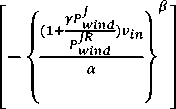
References Multi-Objective Optimal Dispatch Solution of Solar-Wind-Thermal System Using Improved Stochastic Fractal Search Algorithm
- J Nanda., D.P. Kothari, K.S Linga Murthy, “Economic emission load dispatch through goal programming techniques”, IEEE Trans. on Energy Conversion 3(1), (1988) 26-32
- C Palanichamy, N.S Babu, “Analytical solution for combined economic and emissions dispatch”, Electric Power System Research 78, (2008) 1129–1137.
- M Basu. “Economic environmental dispatch using multi-objective differential evolution”Applied Soft Computing 11, (2011) 2845–2853
- M S Kaurav, H M Dubey, M Pandit, BK Panigrahi,Simulated annealing algorithm for combined economic and emission dispatch,in proc. IEEE Inter. Conf, ICACCN 2011,pp. 631-636.
- B.K Panigrahi, R.V.Pandi, S. Das, S.Das, “Multi-objective fuzzy dominance based bacterial foraging algorithm to solve economic emission dispatch problem” Energy 35, (2010) 4761-4770.
- N.Pandit, A. Tripathi, S.Tapaswi, M Pandit, “An improved bacterial foraging algorithm for combined static/dynamic environmental economic dispatch”Applied Soft Computing 12, (2012) 3500–3513.
- P K Roy, Sudipta Bhui “Multi-objective quasi –oppositional teaching learning based optimization for economic emission load dispatch problem”, Electrical Power and Energy systems:53(2013):937-948.
- U. Güvenç, Y.Sönmez, S.Duman, N.Yörükeren, “Combined economic and emission dispatch solution using gravitational search algorithm” Scientia Iranica D vol.19 no.6 pp.1754–1762 (2012)
- K.Bhattacharjee, A.Bhattacharya, S.H.Dey “Solution of Economic Emission Load Dispatch problems of power systems by Real Coded Chemical Reaction algorithm”, Electrical and Energy systems vol.59,pp.176-187,(2014)
- K.Bhattacharjee, A.Bhattacharya, S.H.Dey, “Backtracking search optimization based economic environmental power dispatch problems”. Electrical Power and Energy systems 73, 830-842. (2015)
- A J Wood, B F. Wallenberg, “Power Generation, Operation and Control”. 1984, New York: Wiley.
- J. Hetzer, D. C. Yu, K. Bhattarai, “An Economic Dispatch Model Incorporating Wind Power”, IEEE Trans. On Energy Conversion, vol. 23, no. 2, pp. 603-611, 2008.
- X. Liu, “Economic Load Dispatch Constrained by Wind Power Availability: A Wait-and-See Approach,” IEEE Trans. Smart Grid, vol.1, no.3, pp. 347-355, 2010.
- H. M Dubey., M.Pandit, B.K Panigrahi, “Hybrid flower pollination algorithm with time-varying fuzzy selection mechanism for wind integrated multi-objective dynamic economic dispatch”,Renewable Energy, 83,188-202 (2015).
- S. H. Karaki, R. B. Chedid, R. Ramadan, “Probabilistic Performance Assessment of Autonomous Solar-Wind Energy Conversion Systems”, IEEE Transactions on Energy Conversion, Vol. 14, No. 3, September 1999. pp. 766-772
- H. Bilil, G. Aniba, M. Maaroufi, “Probabilistic Economic Emission Dispatch Optimization of Multi-Sources Power System”, Energy Procedia 50 (2014) 789 – 796.
- M. Fadaee, M.A.M. Radzi, “Multi-objective Optimization of a stand-alone hybrid renewable energy system by using evolutionary algorithms: A review”, Renewable and Sustainable Energy Reviews 16 (2012) 3364–3369.
- H.Salimi,“Stochastic fractal search: A powerful metaheuristic algorithm”, Knowledge based Systems 75,(2015) 1-18.
- J Kiefer, "Sequential minimax search for a maximum", in Proceedings of the American Mathematical Society 4 (3), 1953, pp. 502–506.
- M.K. Deshmukh, S.S. Deshmukh, “ Modelling of hybrid renewable energy systems”, Renewable and Sustainable Energy Reviews 12 (2008) 235–249
- Solar Radiation Hand Book (2008), A joint Project of Solar Energy Centre, MNRE Indian Metrological Department
- K. Deb, “Multi objective optimization using evolutionary algorithms”, Jhon Wiley & Sons, 2001.
- C.L Hwang, K. Yoon, “Multiple attribute decision making: Method and applications”, Spinger-Verlag,New York,NY, 1981.
- M. Behzadian., S.K.Otaghsara., M.Yazdani, J. Ignatius, “A state of art survey of TOPSIS applications”, Expert system with application.39,13051-69 (2012)
- A. Layeb, S. R. Boussalia, “A Novel Quantum Inspired Cuckoo Search Algorithm for Bin Packing Problem”, I.J. Information Technology and Computer Science, 4(5), 58-67, 2012.
- M. Orouskhani,Y. Orouskhani,“A Novel Cat Swarm Optimization Algorithm for Unconstrained Optimization Problems”, I.J. Information Technology and Computer Science, 5(11), 32-41, 2013.
- D.N. Le, “A New Ant Colony Optimization Algorithm Applied to Optimizing Centralized Wireless Access Network” I.J. Information Technology and Computer Science,6(4), 30-36,2014.
