Multiresolution Fuzzy C-Means Clustering Using Markov Random Field for Image Segmentation

Published Online October 2009 in MECS

Segmentation has been found extensive applications in areas such as quantitative analysis of brain tissues, scene analysis, content-based image retrieval and object tracking[1,2]. The purpose of image segmentation is to partition the given image into a number of regions with significantly different properties, such as statistical and structural information. Segmentation is implemented by assigning each pixel to one of a finite number of classes or labels, based on certain contextual property of the neighbouring pixels.

Manuscript received Febuary 13, 2009; revised July 25, 2009; accepted September 15, 2009.

corresponding author: Xuchao Li

In recent years, image segmentation technique based on stochastic field model has received extensive attention, one of the most influence on image segmentations is Markov random field (MRF)[3]. It is roughly classified into three types, namely, the single resolution and multiresolution segmentation based space domain [4, 5], multiresolution segmentation based wavelet domain [6].

The single resolution segmentation approach assumes that the spatial distribution of regions consists of a single random field, the feature field based on original image is described by conditional probability function given a label field, the label field is modeled as MRF to impose smoothness constraints on the image segmentation [7]. The technique based on single resolution has demonstrated substantial success for image segmentation, but the single resolution MRF model usually favors the formation of large regions and leads to over segmentation, although the segmentation performance can be improved by using a larger neighborhood for each pixel, it maybe blurs the high frequency of image, these shortcomings produce unfavourable influence on image analysis.

The multiresolution segmentation based space domain [8] assumes that the spatial distribution of regions consists of a serial of random field models from coarse to fine scale, the coarse scale label field affects the fine scale label field by the interscale label transition probability of MRF. The approach takes into account the interscale contextual information of pixels, it can improve the accuracy of boundary localization, but when the image is blurred by noise, the spatial domain multiresolution approach will lose the performance of region classification and boundary detection. Although spatial filter can reduce the effect of noise, but the high frequency information of image is badly worn out. Moreover, the feature field model is still established by probability density function (pdf) of pixels, which can not accurately capture the wide range frequency features of image. Since image has locally varying statistical distributions such as texture regions, smooth shading regions, flat regions or their combinations of aburt features, the spatial non-stationary feature contradicts single frequency statistical characterization based on pixels.

The multiresolution segmentation based wavelet domain receives extensive attention. Wavelet transform decomposes an image into a casual hierarchical subimages, which are characterized by a serial of MRF models with good time-frequency characteristics[9]. The approach can incorporate the interscale persistence and intrascale clustering properties of wavelet coefficients into the label field prior probability model, it can overcome the shortcoming that the label prior probability model easily produces over segmentation. Moreover, wavelet transform can reduce noise without smearing high frequency information of image, since the features of image are extracted by high pass and low pass filter with different frequencies, the filter bank adapt to the non-stationary characterization of image.

In the last decade, soft computing approaches, such as k-means, possibilistic c-means (PCM)[10] and fuzzy c-means (FCM) clustering[11], have been successfully used for image segmentation. K-means forces each pixel to be associated with exactly one label, it is not realistic, since the uncertainty is almost everywhere in medical image, particularly in the case of magnetic resonance image (MRI) due to partial volume effects and noise (during the acquirement). Consequently, the labels of border between tissues can not be thought as belonging to a single region and must be determined by the degree of membership, fuzzy method is a strong tool to solve the problems.

PCM clustering algorithm[10] is firstly proposed by Krishnapuram Raghu and Keller James M. in 1996, it is a variant FCM algorithm, the PCM objective function is constructed by the Euclidean distance between the likelihood function of sample and clustering centers, the algorithm can overcome the unfavourable influence of noise or outliers on image segmentation. But the difficulty of the algorithm is how to determine the likelihood function of characterizing samples and cluster centers, and how to incorporate spatial constraint into the objective function, which directly affects the segmentation results. Moreover, PCM algorithm is sensitive to initialization, it is usually initialized by the standard FCM algorithm.

The first studied FCM algorithm by Jim Bezdek [12], who constructed FCM objective function for image segmentation, but the algorithm has some limitations, firstly which is sensitive to noise, noise can be reduced by the chosen space filter groups, but the edges of image is seriously lost. Secondly, lacks of spatial context information constraints, the spatially neighboring pixels maybe belong to the same region that can be of great aid in image segmentation. Thirdly, is sensitive to initial values and easily converges a local maxima.

In order to overcome the shortcomings of standard FCM clustering and PCM algorithm without taking into account spatial constraints, many researchers have incorporated local spatial statistical information into the conventional clustering algorithm[13] to improve the performance of image segmentation by modifying the objective function, but the improved objective function is established in single or multiresolution space domain[14] instead of wavelet domain.

In this paper, a wavelet domain MRF and FCM clustering algorithm with spatial constraints for robust multiresolution image segmentation is proposed, it has the following features:

The given image is decomposed into different subbands, which can reduce noise and accurately extract the features of image. In order to represent the observed image for multiresolution Bayesian segmentation, we construct a serial of feature field and label field models.

At the initial label determination of wavelet coefficient stage, the feature field is described by Gaussian mixture model (GMM)[15], it can provide a good fit to the global statistical distribution of wavelet coefficients. In order to capture the intrascale clustering and interscale persistence properties of local wavelet coefficients, the contextual statistical information of intrascale and interscale label field models are captured by Markov prior probability model, the model parameters are estimated by improved expectation maximization (EM), according to maximum a posterior (MAP) estimate, the initial label of wavelet coefficient across scales is determined. Taking advantage of the initial label of wavelet coefficient, we can obtain initial clustering centers and the degree of membership for the following improved FCM algorithm.

At the image segmentation stage, we incorporate the local statistical distribution and contextual information of wavelet coefficients into the FCM objective function, the local statistical information captures the clustering property of intrascale wavelet coefficients, the contextual information captures the persistence property of interscale wavelet coefficients. We optimize the modified FCM objective function, an unsupervised multiresolution image segmentation algorithm from coarse to fine scale is obtained.

The rest of this paper is organized as follows: In section 2, two-dimensional discrete wavelet transform (DWT) of image is briefly introduced, then the feature field of image is described by GMM, the intrascale and interscale contextual information is captured by MRF, the model parameters are estimated by improved EM algorithm, according to MAP rule, the initial label of wavelet is determined. Section 3 gives the modified FCM objective function, which incorporates the intrascale clustering and interscale persistence properties of wavelet coefficients, optimizing the new objective function, an unsupervised image segmentation algorithm is obtained. The proposed is outlined in section 4. Simulation results on real MRI and peppers image with noise are given in section 5, and some conclusions are drawn in section 6.

• II.    The initial label determination of wavelet

COEFFICIENT

• A.    Image Multiresolution Representation by DWT

Wavelet transform is a multiresolution analysis technique that has been developed and applied in various fields, such as astronomy, finances, quantum physics, signal processing, video compression and image processing[16,17], etc. Wavelet has a varying window size and finite duration to fit low and high frequency information of non-stationary signals, and produces an optimal time-frequency resolutions from coarse to fine scale [18].

The continuous wavelet transform of a 1-dimensional signal f ( x ) is defined as

Wf ⁽ a , b ) = ( f , ф ⁽a , b )) = J R f ⁽ xMb ⁽ x)dx , ⁽¹⁾ , ,¹ ( x — b

Ф а.Ъ ⁽ x) = l a i 2 P ^“ a “ j . ⁽²⁾

Where, a is called scale parameter that controls wavelet frequency, b is called translation parameter that controls wavelet position (time), ^Q denotes inner product. The function ф _аЬ is called mother wavelet, which satisifies J ф _а b ( x ) dx = 0 and generates the other wavelet functions with parameters a dilation and b translation.

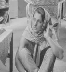
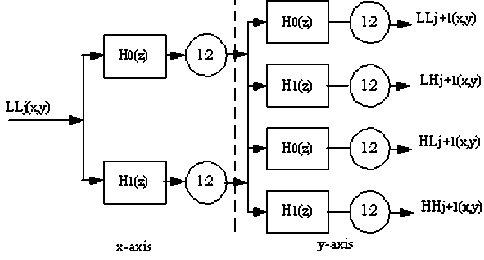
The two-dimensional wavelet transform is performed by consecutively convolving one-dimensional filter bank with the rows and columns of image. The given image is decomposed by applying low-pass and high-pass filters associated with a mother wavelet as shown in Fig.1. H0(z) and H1(z) denote the one-dimensional low-pass and high-pass filters, respectively, while 1:2 represents downsampling by a factor of 2 in horizontal and vertical direction of image. Fig.1 shows four subband images with N/2j x N/2j resolution in j-level wavelet transform, LLj denotes approximate subimage, we can recursively decompose it further to obtain next level multiresolution representation of the original image, and three subimages, LHj, HLj, HHj denote the horizontal, vertical and diagonal subband details. Fig. 2(b) shows that the image DWT decomposition and wavelet coefficients distribution. The given image is decomposed by three level wavelet transform in Fig.2(b), as can be seen, the wavelet transform preserves better the spatial-frequency features of image. As far as frequency property of wavelet coefficients is concerned, the stationary portions of image is described by a few large magnitude value wavelet coefficients. Moreover, the magnitude do not vary significantly across scales. On the contrary, the non-stationary portions (around edges) of image is described by large magnitude value wavelet coefficients. As far as spatial property is concerned, the spatially relative position of wavelet coefficients remains unchange from coarse to fine scale. In other words, the persistence of wavelet coefficient magnitude propagates across scales, the property indicates the label of interscale wavelet coefficient maybe remains unchangeable. In Fig. 2(c), the subimages of three level wavelet transform can be represented by hierarchical structure, each coefficient in coarse scales has four wavelet coefficients in the next finer scale, as the pink color box shows the relationship between “parent” and its four “children”. According to the persistence property of interscale wavelet coefficients, it indicates that the label of children is closely similar to its immdeiate parent. Fig.2(d) shows the statistical distribution of the HH2 subband wavelet coefficients, it means that intrascale wavelet coefficients have clustering and compaction properties, the label of each wavelet coefficient depends on its direct neighbouring wavelet

Figure 1. Tree representation j-scale DWT decomposition

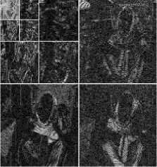
(b) three scale DWT decomposition

coefficients.

(a) original image

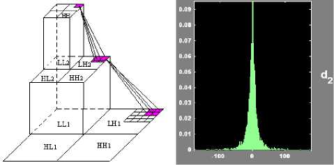
(c) subband hierarchical representation (d) coefficients distribution Figure 2. Image DWT decomposition and coefficients distribution

• B.    Establishment of Feature Field Statistical Model

After the given image is decomposed by wavelet transform, we are interested in subimages of wavelet domain instead of the spatial domain where the original image exists. Because of multiresolution time-frequency property of wavelet transform, subband wavelet coefficients reflect the statistical features of subimages. Fig. 2(d) displays the histograms of wavelet coefficients of the HH 2 subband of the original image, the wavelet coefficients exhibit approximately Gaussian statistics, GMM[15] can approach arbitrary pdf. To better model the subband statistical features of wavelet coefficients, we utilized GMM for approximating the histograms of wavelet coefficients. According to the decorrelated property of wavelet coefficients, we can assume that coefficients subbands are conditionally independent, the model likelihood of wavelet coefficients is expressed as the following product

N /2 ^j × N /2 ^j

f ( ω | θ ) = ∏ f ( ω k | θ k )                  (3)

k = 1

Assuming that the image consists of M distinct regions, the model likelihood function of wavelet coefficient is approximated by GMM with M components, it is defined as

M f ( ω k | θ k ) = ∑ π k^m g ( ω k , θ k^m ) m = 1

Where, π _k ^m is the mixture ratio of the m - th component g ( ω _k , θ _k ^m ) of GMM and satisfies

M

∑ π _k ^m = 1 , 0 ≤ π _k ^m ≤ 1 , 1 ≤ m ≤ M             (5)

m = 1

The conditional likelihood model of wavelet coefficient given the label can be formulated as following

g ( ω k | l k^m , θ k^m ) =

exp[ - 12( ω k - µ k^m ) σ k ^{- 2( m )} ( ω k - µ k^m )]

2 πσ _k ^m

Where, 0k = {w™ .ofm), m = 1,2, ™, M}, Ц and ст2(m) are mean and variance.

Thus the overall subband wavelet coefficients distribution of image is parameterized as follows

0 j = К , W m X^{( m} ) , k = 1,2, l , N /2 j x N /2 j ; m = 1,2, l , M }

Where j denotes scale, B denotes wavelet coefficient three subbands.

• C.    MRF Theory in Wavelet Domain

From (3) and (4), the histogram of wavelet coefficients can be approximated by GMM, but GMM only describes wavelet coefficients frequency statistical property, the spatial interactions between wavelet coefficients is not considered. Wavelet coefficients reflect the spatial-frequency information of image, subband wavelet coefficients from totally different two images maybe have the same frequency histogram, however, the spatial structure information of images is totally different. In order to characterize the spatial structure of image, we exploit MRF to describe the local interactions of wavelet coefficients.

After the image is decomposed by J-level wavelet transform, we obtain 3J+1 subimages. It is assumed that the subimages are defined on a serial of subband lattics S = {S', SB-1v, S4}, Sb = {SHH1, SHL, SLLH'}, SHH- = N/2j ×N/2 , N × N represents the size of original image. Let L denote the random field associated with the labels of the subimages, it is defined as L = {lLLJ,IB4,l,IB1} , BHHHLLH l = {l ,l ,l }. Let η denote neighborhood system of sites, it is defined as n = {nLLJ ,nBJ -1,^,ПВ1} , ηB = {ηiB ,i∈SB }, where, ηiB is the set of sites neighboring i , i ∉ηiB and i ∈ηkB ⇔k∈ηiB . A random field L is regarded as an MRF on S with respect to a neighborhood systemη, the random field is defined as

p ( l _i ^B | l _{ ^B _η ^jB _{- i }}) = p ( l _i ^B | l _k ^B , k ∈ η _i ^B )                       (8)

According to Hammersley-Clifford theorem[19], a given random is an MRF if and only if its probability distribution p(liB )is a Gibbs distribution, the probability distribtion of the label field is formulated as

p ( l i^B ) = _Q ¹ exp[ U ( l i^B )]                           (9)

Where, Q is a normalizing constant (partition function), U ( l _i ^B ) is the energy function having the following form

U ( l i^B ) = ∑ V k ( l i^B )                          (10)

k ∈ η _i ^B

• D.    Establishment of Intrascale and Interscale Label Field Prior Probability Model

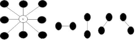
As we see from Fig. 2(d), the wavelet coefficients have clustering and compression properties. From Fig. 2(b), we can know the neighbor wavelet coefficients maybe have the same labels, so when determining the label of wavelet coefficients, we must consider the influence of intrascale wavelet coefficient labels. To take intrascale spatial context information into account, we adopt MRF prior probability model for imposing the interactions of wavelet coefficient label field. The prior probability model should express the belief that the pixels within a region have a higher probability. We use the second-order neighbourhood system with respect to the Euclidian distance, and only consider the interactions of wavelet coefficients with two pair site clique, as is shown in Fig.3.

(a) (b)

Figure 3. Intrascale neighbourhood and clique. (a) A second-order neighbourhood system with respect to the Euclidian distance. (b) The four associated two-site cliques.

According to (9), the label field prior probability model of intrascale wavelet coefficient is defined as

p ( l v ) = [exp( U ( l v ))] / Q 1                 (11)

Here, Q ₁ is a normalizing constant called the partition function, v denotes the position of sublattics. U ( l_v ) is called the intrascale energy function, which has the following form:

U ( l v ) = ∑ ∑ V τ ( l v )              (12)

v _∈ s^B τ ∈ η ( v )

Where v ∈ s ^B , η ( v ) is the second order neighbour system, V _τ ( l_v ), which only depends on l_v , τ ∈ η ( v ), are the clique potential function. The function has the following form

V τ ( l v ) = - β ∑ ∑ [ δ ( l v - l τ ) - 1]          (13)

v _∈ s^B τ ∈ η ( v )

Where, the Markov parameter β controls the spatial interactions of local wavelet coefficients, so that two neighbouring wavelet coefficients are more likely to have the same label than the different labels. 5 ( D ) is the discrete delta function, it is defined as

5 ( l a - l b ) =

if ( l a = l b ) if ( l a * l b )

Fig. 2(b) indicates the interscale wavelet coefficients have persistence property. Fig. 4 shows a wavelet coefficient is decomposed by 3-level wavelet transform, each wavelet in coarse scale has four children in next fine scale. If we want to determine the label of node v at j-th scale, according to the interscale persistence property, the label of its parent node 5 in (j-1)th scale will affect the label of node v , moreover, node 5 has three brothers, which derive from the same parent node 1, their labels will affect the label of node v . We call the nodes of 2,3,4 and 5 as the interscale neighbor of node v . It is assumed that the labels of interscale wavelet coefficients have one order Markov property, The prior probability model of interscale label field with quadtree neighborhood system is defined as

P ( lB\l B ^-) = "1exp[ - ^ 2 ( l B )]               (15)

Q ₂

Where, U ₂( l _v ^{B j} ) is called the interscale energy function, it is defined as

U 2 ( l B ) = -a X X [ 5 ( l B - l B ^{- 1} ) - 1]        (16)

v E S B 7 E p ( S B' -1 )

where a denotes the Markov parameter, p ( s B ' ^{- 1}) denotes the interscale neighbour clique.

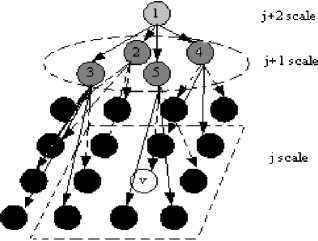
Figure 4. Interscale neighbourhood and clique

• E.    MAP Estimate of Initial Label

The purpose of multiresolution image segmentation is to assign a class label from the set of L for each subband wavelet coefficient. Let l$ denote the optimum estimate for true but unknown label l* of wavelet coefficient, l$ and l* are realization of MRF, which are formulated as Markov label field prior probability model. The observed subband wavelet coefficients o are formulated as a realization of GMM, which is formulated as feature field conditional probability model given the label field. According to MAP, the optimum criterion of label is formulated as l = arg max p (l| o, 0)

l E L

Where 0 is the model parameter.

Using Bayesian rule, equation (17) is reformulated as

$ = arg max p ( l | o , 0 ) p ( l )                      (18)

l E L

From (18), we need to compute the prior probability of label field and the likelihood probability of feature field. Submitting (6), (11) and (15) into (18), according to MAP equivalent to minimizing energy function, (18) can be expressed as

U ( 1 1 o ) = argmin[ U ( o | 1 ) + U 1 ( l ) + U ₂ ( l )]           (19)

l E L

Where U ( 1 | o ) denotes the posterior energy function of label field.

Submitting (6), (13) and (16) into (19), according to the local property of MRF, the posterior energy function is expressed as

U(lv I ln(v),o) « У    11[lnCk + ° -^)2 ] + в 2

TEn(v),YEp(S ' ) I

в[5(lv — It ) — 1] + a[5(lv -1,) -1]}

Some stochastic iterative optimization algorithms such as simulated annealing and deterministic relaxation are adopted to get the global minimum of (20), but finding the optimum labels of the posterior energy function requires a lot of compution time. In this paper, we adopt the iterative conditional modes (ICM) algorithm[19] to update the label of wavelet coefficient. Given the wavelet coefficient o and the initial label of coarse scale wavelet coefficient, the ICM algorithm sequentially updates label lv^{1 + 1)} by minimizing the following formula

( 1 +1)                                           / 4

l v = argmin U ( l v | l n (),, , o ) .               (21)

Where t denotes the numbet of iterations.

• F.    EM Algorithm for Model Parameters Estimation

To implement image segmentation, the parameters 0 in GMM have to be estimated, the procedure for determining the unknown parameters is known as model fitting, the objective of model fitting is to obtain the unbiased estimation of model parameters. However, because of the nonlinear relationship between the parameters of GMM and their pdfs in (4) and (6), it is impossible to derive an explicit expression for the maximum likelihood (ML) estimation of parameters. Many iterative algorithms have been employed to solve the problem, among which the EM algorithm[20] is the one most widely utilized.

The classicla EM algorithm is a general ML estimation algorithm, it has a well-known basic structure for dealing with the incomplete data, its concrete structure is problem dependent. Here, the determination of wavelet coefficient label is formulated as an incomplete data processing problem. The observed wavelet coefficient o is considered as the incomplete data characterized by likelihood p ( o | 0 ) , let the label l denote unobservabel or missing data, let the couple ( o , l ) denote the complete data characterized by the joint likelihood function p ( o , 1 1 0 ) , where 0 is parameter to be estimated. The ML estimation of 0 is determined by the following formula

0 = arg max log p ( o , 11 0 )                (22)

EM algorithm starts with assigning initial values to the parameter 0 , it then iteratively alternates between the expectation step (E-step) and maximization step (M-step)

for approximating the ML estimation of parameter θ . It can be expressed as follows:

E-step: computing the log-likelihood function conditional expectation of the complete data z , given the observed wavelet coefficient ω and the current parameter θ ^{( t )} ML estimation

Φ ( θ | θ ^{( t )} ) = E _l [ln p ( ω , l | θ ) | ω , θ ^{( t )} ]               (23)

Where E l [ □ ] denotes the mathe expectation of random variable l , which is described by the conditional pdf of missing data given the wavelet coefficients.

M-step: the parameter θ is reestimated by maximizing θ ^{( t + 1)} = argmax Φ ( θ | θ ^{( t )} )                  (24)

θ

Where t denotes the number of iterations.

From (24), we can get ML estimation of parameter, equation (23) indicates that the ML estimation of parameter is seriously dependent on initialization, consequently, clssicial EM algorithm usually obtains the local maxima. Besides, because EM algorithm is a general framework, we must integrate concerte application issue into the general framework for obtaining the optimum estimation of parameter. To improve the performance of parameter estimation, we introduce histogram of image as constraint conditions of EM algorithm.

In order to impose constraints, we introduce a hidden variable z , let z = { z_p = [ z_pX , l = 1,2, ™ , L ], p = 1,2, ™ , P} , where z _pl denotes the probability of grey level p belongs to the l th region, P denotes the number of grey levels. The improved EM algorithm computes the conditional expectation of the complete data ( ω , z ) as follows

Φ ( θ | θ ^{( t )} ) = ∫ p ( z | ω , θ ^{( t )} ) • ln p ( ω , z | θ ) dz         (25)

From (25), we do not have any prior knowledge about missing variable z , in order to compute the conditional expectation of complete data, we must obtain the prior probability of missing data z via maximum entropy principle. The maximizing entropy of prior probability of missing data z is defined as

H =- ∫ p ( z | ω , θ ) • ln p ( z | ω , θ ) dz            (26)

Under the constraint

∫ p ( z | ω , θ ) dz = 1                        (27)

Equation (27) indicates the constraint must conform to the normalising conditon.

According to Lagrangian theorem, the optimization is to maximize the following objective function

E=Φ(θ|θ(t))+ΓH+λ(∫ p(z|ω,θ)dz-1)

Where Γ and λ are Lagrange multipliers.

By maximizing (28) with respect to the prior probability p ( z | ω , θ ) , we have

p(z) = 1 [p(ω, z|θ)]Γ

Q ₃

Where Q ₃ is the normalising function that satisfies

Q3 =∫z[p(ω,z|θ)]Γdz(30)

In (29), we introduce a parameter Γ , which is similar to the temperature parameter of simulated annealing algorithm, during the cooling process, we can get the global optima. The improved EM algorithm is formulated as:

E-step: the conditional expectation of complete data ( ω , z ) is

Φ ( θ | θ ^{( t )} ) = ∑ ^{[ p ( ω , z | θ )] Γ} • ln p ( ω , z | θ )     (31)

z ∑ [ p ( ω , z | θ )] ^Γ

z

M-step: the parameter θ is reestimated by maximizing (31).

Ш. Fuzzy Clustering Algorithm With Spatial Constraints

According to (21), we obtain the initial labels of wavelet coefficients from coarse to fine scale, then the initial cluster centers of regions are determined. In order to overcome the standard FCM algorithm without considering wavelet domain spatial-frequency property shortcomings[21], we incorporate intrascale local spatial clustering property and interscale frequency persistence property into FCM objective function. The improved FCM objective function is optimized by Lagrange multipliers, we can obtain a new image segmentation algorithm by iteratively updating clustering centers and degree of membership. Taking advantage of maximizing degree of membership criterion, the final segmentation results of original image are obtained.

• A.    Standard FCM Algorithm

The FCM algorithm assigns each wavelet coefficient to a region label by using fuzzy degree of membership. Let <У = {^sj , j = 1,2,™, J} , ^s = {^s_7 , ^sj ,™, ^sj } , ^sj e ^ , denote the j th scale wavelet coefficiens to be partitioned into K classes, and the grey value C = {CsJ , J = 1,2,L, J} , c , = { c 1,,c2,,™,cK}, c , ec , denote a set of the region sj              sjsj sj sj cluster centers. In order to achieve optimum clustering, the formulation of the FCM optimization model to be minimized is defined as follows

J m ( u , c ) = ∑∑ ^K ( u _s ^{i ,} j ^l ) ^m ω _s ⁱ j i ∈ s ^j l ^{= 1}

with the following constraints

• ^L u ^{i , l} = 1 , 0 ≤ u ^{i , l} ≤ 1 s ^j           ,              s ^j

l = 1

- c s^l j ²

where usi,jl denotes the degree of membership of wavelet coefficient ωi in the lth cluster, cl is the lth sj                                                   sj class center, • represents the Euclidean distance, andm is a fuzzifizer that controls the resulting partition, m ∈ [1, ∞) .

• B.    The Intrascale FCM Objective Function

In standard FCM algorithm, the degree of membership is dependent solely on the distance between the wavelet coefficient and each individual cluster center in wavelet domain, and disregards the spatial property of wavelet coefficients. According to the spatial clustering property of intrascale wavelet coefficients, the local neighboring wavelet coefficients usually possess similar features, the probability that they belong to the same region is great. In order to capture the spatial clustering property, the intrascale FCM objective function is defined as

K 2

JN (jm (U, С) =     Z Z (4 j*) m K (Pj ) - 4(

1              NRi G N (ms) l =1

where N(pj) stands for the set of neighboring wavelet coefficients around p, , N„ stands for the size of window, sj        R, and the other parameters are of the same meaning as those in (32).

• C.    The Interscale FCM Object ve Funct on

Wavelet transform has spatial-frequency property, in (34), we incorporate the local spatial clustering property into the FCM objective function, Fig.2(b) shows that wavelet coefficient has the interscale similar frequency persistence property, the label of child in fine scale is similar to that of its parent’s neighbors in coarse scale. In order to capture frequency persistence property, the interscale FCM objective function is defined as

J-p j xf' c ) = Z Z ( u ,' -| ^m„. ,,)- c . |‘    (35)

"                    i g p ( m ", -, ) ^l = 1                       ■'

Where p ( p j ,) denotes the set of neighbors of m j in the ( j - 1)th scale, m ' j -, is the immediate parent of m ' j in the j th scale, p_{p ( m} i ) denotes the neighboring wavelet coefficients of m ' j -, in the ( j - 1)th scale, and the other parameters are of the same meaning as those in (32).

• D.    Local Statistical Fuzzy Degree of Membership

The degree of membership in standard FCM algorithm only depends on the distance between wavelet coefficient and cluster center. In this paper, we incorporate the interscale persistence and intrascale clustering property of wavelet coefficient into the standard FCM objective function, consequently, the degree of membership of new FCM algorithm must change accordingly. According to the spatial-frequency feature of wavelet transform, the intrascale clustering and interscale persistence property of wavelet coefficients is incorporated into the degree of membership, which is defined as

( uV ) * = uVp , , „( m ' J                      (36)

s ^j            s ^j -^r[ N p ( m , )] s ^j

Under the following constraint

0 <  ( u ' j ) * <  1 , Z ( u ' j ) * = 1                        (37)

Where N p ( p _t ) = N( m^: ) + p ( p j -1 ) denotes the intrascale two order neighbors and interscale parent neighbors of wavelet coefficient m _s ⁱ j , the intrascale spatial and interscale frequency statistical information p , ( m i j )

[ Np (m,j)] s is expressed as p ,  (mi,) =

[ N p ( m sj )]^V s^; '

( A + B ) • p ( m i j ll n )

Z   P (m^ll n ) +    Z    P P>lk )

^m n ^G N ( ^m i )                     ^m n ,^G p ( ^m i ,)

sjsj                                   sjsj

where, 5 ( D ) is sample function, A = Z ^ ( P l n ) P( m n I l n ) , m n g N ( p , )

в = Z     5 ( l . - 1 „ ) P( m n j ll n ) .

p , -1 ^G p P - )

• E.    Improved FCM Objective Function

The standard FCM algorithm in (32) does not impose any spatial-frequency constrain on objective function, which can lead to forming small undesirable regions. The objective functions in (34) and (35) take into account the intrascale clustering and interscale persistence property of wavelet coefficiet, respectively. Submitting (36) into (32), (34) and (35), the modified FCM objective function in wavelet domain can be written as

J^U * , C ) = J m ( u * , c ) + A J ( u * , c ) + ^ 2 J ( u * , c ) (39) s^js^j

Where the parameter A 1 is a weight that controls the intrascale spatial context information, A 2 controls the interscale persistence information.

• F.    Opt m zat on Improved FCM Object ve Funct on

The segmentation algorithm is formulated as minimizing (39) under condition (37), the optimization of (39) will be solved by using Lagrange multiplier technique

J M ( U * , C ) = J m ( u * , C ) + A 1 J n ( m i ), m ( u *, C ) + A 2 J p (^,m ( u * , C ) s^js^j

K

+ A , (1 - Z u * 1 ^{i , l} ) )

l = 1

The derivative of (40) with respective to us*(j ,l) and cslj respectively. The modified fuzzy c-means objective function of JM* (U,C) can be minimized iteratively by updating membership degree and clustering centroids equation respectively

||m'j - c'j II + ^11|mN(к, ) - c' I + ^2 Ipp(к,- ) - c'j I m-1

^P N p ( m i ) s^j

W. Overview of The Proposed Algorithm

The complete procedures from the optimum label establishment to the final modified FCM segmentation algorithm can be stated as follows

• A.    Determining the label of wavelet coefficients procedure

• (1) . Feature extraction: performing J level wavelet decomposition of the input image.

• (2) . Estimating GMM parameters by improved EM algorithm.

• (3) . According to Bayesian rule, calculating the label of wavelet coefficient using (21).

• (4) . Given the label of wavelet coefficient, we can get the conditional probability p ( ω _s ⁱ j | l _n ) . Submitting p ( ω _s ⁱ j | l _n ) into (38), we can calculate the wavelet coefficient spatially statistical information of p .

p Nρ ( ωⁱ )

s ^j

• B.    The modified FCM segmentation algorithm procedure

• (1) . According to the results of the j-th scale wavelet coefficient label estimation, setting the number of clusters, initializing the fuzzy membership function u _k ^j _, ⁽ _l ⁰⁾ , u k^j ,⁽ l ⁰⁾ ∈ [0,1] .

• (2) . Computing membership functions using (41).

• (3) . Calculating the fuzzy cluster centers using (42).

• (4) . if u _k ^* _{, i} ^{( τ + 1)} - u _k ^* _{, i} ^{( τ )} ≤ ε stop; otherwise go to step

B(2). Here, τ represents the number of iterations.

V. Simulation Results

We have tested the proposed algorithm via two different images, one is real MRI image, another is a peppers image with noise. In order to evaluate the performance of image segmentation, we compare our simulation results with that of the other segmentation algorithms, standard FCM algorithm and FGMM-MRF model based on single resolution.

Fig.5 shows the segmentation results by applying three different algorithms to MRI image. Fig.5(b) shows the segmentation results using standard FCM algorithm, it produces a lot of isolated regions, because standard FCM algorithm does not take into account the spatial context information of pixels. Fig.5(c) shows the result using FGMM-MRF algorithm, the segmentation result is better than that of FCM algorithm, because the FGMM-MRF algorithm captures the local pixel interactions by MRF prior probability. However, it still produces a few isolated tissues, because the feature model is dependent on single resolution pixels of space domain, which is very difficult to describle the nonstationary property of image. Fig.5(d) shows the segmentation results using the proposed algorithm, the result is better than the others, such as producing few isolated issues, the accuracy of classifying different tissues and edge location.

Fig.6 shows the segmentation results by applying three different algorithms to peppers image with noise. Fig.6(b) shows that FCM algorithm is sensitive to noise, the regions are misclassified seriously. Fig.6(c) shows that FGMM-MRF algorithm based on space domain is still sensitive to noise, and produces a lot of isolated regions. Fig.6(d) shows that the proposed algorithm based on wavelet domain is insensitive to noise, the segmentation result is encouraging, such as reliable edge location and the accuracy of differentiating different regions.

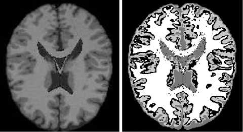
(a) MRI image

(b) FCM segmentation

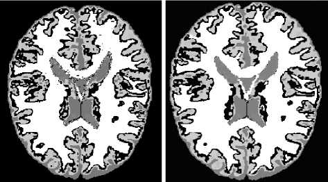
(c) FGMM-MRF

(d) the proposed method

Figure 5. Comparison of segmentation results on MRI

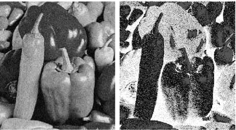
(a) MRI image

(b) FCM segmentation

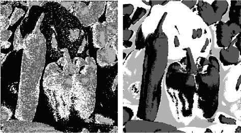
(c) FGMM-MRF

(d) the proposed method

Figure 6. Comparison of segmentation results on peppers image

И . Conclusion

In this paper, a new multiresolution technique for image segmentation based on wavelet domain spatial-frequency MRF and modified FCM algorithm with interscale and intrascale context constraints is proposed. The multiresolution image segmentation algorithm contains the determination of initial label of wavelet coefficient from coarse to fine scale and image segmentation steps. At the determination of initial label stage, the statistical distribution of feature field in wavelet domain is captured by GMM, the interscale and intrascale label field prior probability models are characterized by MRF, taking advantage of Bayesian rule, the initial label of wavelet coefficient from coarse to fine scale is determined. At the image segmentation stage, a modified FCM objective function is established, it incorporates intrascale clustering and interscale persistence properties into the standard FCM objective function, optimizing the new objective function, an iterative image segmentation algorithm is obtained. Experimental results show that the proposed algorithm is more efficient than standard FCM and FGMM-MRF algorithm, such as being insusceptible to noise, reliable edge location and the accuracy of differentiating different regions.

Acknowledgment

This research work is supported by Natural Science Foundation of Jinggangshan University (No. JZ0822); Youth Natural Science Foundation of Jiangxi Provincal Department of Education, China (No. GJJ09589).