Neural Network based Modeling and Simulation of Transformer Inrush Current

Published Online May 2012 in MECS DOI: 10.5815/ijisa.2012.05.01

Inrush current is very important issue for transformer designer. It effects on relay coordination because of ten to twenty times (even more) of rated current during transient period. These abnormal behaviors of inrush current causes relay to operate. Second harmonic based relay discriminate this abnormality in power system [1].Transient period of current (exponential decay) depends on circuit time constant. Transformer is R-L circuit with time constant of L to R. Resistance is very small for large rating of transformer, causes large transient period but it is relatively higher for small rating of transformer and also causes fast decay action in inrush current. Intensity of the inrush current depends on the instance of the sinusoidal voltage in which it is switched on as well as

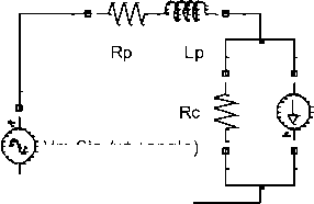
Equivalent circuit of single phase transformer [2] during no load condition is shown in figure 1.

Vm Sin (wt +angle)

Figure 1: Equivalent circuit of Single phase transformer

Inrush Current can be determined by following equations.

Vm Sin (tot + 6 )= (r_p.i ) + ( L_p )+         (1)

‘ = (?Э ⁺ *”          (2)

i m = a Sinh(eX )               (3)

Where r_P, L_P and r_c represents primary winding resistance, primary winding inductance, and core losses resistance respectively. i_m (eqⁿ 3) is magnetizing current.

A. Data collection

Data sets were collected using semi-analytic solution with the help of MATLAB programming. These sets including different values of inrush current at particular remanent flux, magnetizing current, time and switching angle. One data set was prepared for inrush current value based on different value of remanent flux, magnetizing current, and time but at constant switching angle. Second data set was prepared for inrush current’s peak value based on different switching angle and ramanent flux.

Figure 2: Flow chart of ANN Modeling

• A.    ANN Model for Modeling of Inrush current

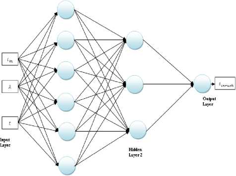
ANN1 structure shown in figure 3 consists of three neurons at input layer ( i_m , λ_n &  t_n ), six and three successive neurons in hidden layers 1 and 2, and one output neuron at output layer ( i_inrush ).

Mathematically, it can be defined by equation 4.

i inrush = ƒ ANN1 (t n , λ n, i m , )

• III.    Case Study

  This study was carried on 120-VA, 60-Hz, (220/120) V transformer [2] and inrush current obtained from equations (1) and (2) using a discrete time, with 83.333μs. The equivalent circuit of this transformer is shown in Figure 1and its parameters (220-V winding) are r_P = 15.4760; L_P = 12 mH; r c =7260Л. For the transformer magnetization curve, as given in equation (3), the following parameters determined experimentally were used: α = 63.084mA; β = 2.43И76" \

• IV.    Neural Network

Neural Network consists of three layers namely input layer, hidden (Processing) layer(s), output layer. Input data fed to network through input layer, after that processing takes place. Output value comes out at output layer which will compare with target value to find out error. Back propagation with LM algorithm is used to minimize this error or reducing tolerance range. Neural Network has beauty to give accurate value depends on input value after well training of network [6,7].The flow chart of modeling of inrush current is accomplished by ANN network is shown in figure 2.Since these data have their own ranges, therefore the data has been normalized at same scale in between 0.1 to 0.9 for well training. Trained Network represents modeling of inrush current. After training, output of network gives normalized values which will convert back to their original values to ensure practical values of inrush current.

Where, n = number of iteration, t n = time, i m = Magnetizing current and λ n = flux linkage.= N. flux

Hidden

Figure 3: ANN1 Structure (3-6-3-1) for Inrush current Modeling

ƒ ANN1 is ANN Structure (3-6-3-1) for inrush current Modeling. Data sets ( i m , λ n &  t n ) were used to train ANN1 so that it able to predict inrush current value based on magnetizing current, flux linkage, and time.

• B.    ANN model for modeling of inrush current’s peak

ANN2 structure shown in figure 4 consists of two neurons at input layer (θ_n , Br_n,) , eight and six successive neurons in hidden layers 1 and 2, and one output neuron at output layer ( i peak, ).

Mathematically, it can be defined by equation 5.

i peakn = f ANN2 в , ВГ п )             (5)

Where n = number of iteration, θ = Switching angle, and Br = remanent flux.

f_ANN2 is ANN Structure (2-8-6-1) for modeling of inrush current’s Peak. Data sets ( 9_n , Br_n ) were used to train ANN2 so that it able to predict inrush current’s peak based on switching angle and remanent flux.

Switching angle is that angle at which transformer gets energized. Switching angle was considered in between 0^o to 180^o.

Remanent flux is that flux which remains in core from switch off to next switch on. As stage of switch on comes, remanent flux will add with flux wave which leads to saturation region of magnetization curve because of adding flux i.e. approximate double of flux which becomes more than maximum flux density of core material. Therefore switching angle and remanent flux plays important role in transformer inrush current.

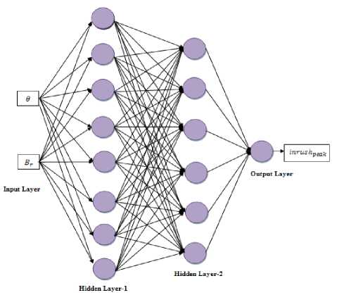
Figure 4: ANN2 structure (2-8-6-1) for modeling of inrush current’s peak

• V. Results and Discussion

• A.    ANN1 Model for Modeling of Inrush current

Inrush current data was obtained using semi analytic solution with assuming maximum initial fluxlinkage value 0.826-Wb coil, and the excitation angle corresponds to θ = 0o. To know accuracy of ANN1 Model, Output data of ANN1 was compared with data which was used to train ANN1 as shown in figures5 and 6.

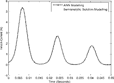
Figure 5: Inrush current with ANN1 Modeling (points) and semi analytic Solution (Line)

Different weights associate with f_ANN1 is described here:

• a)    Weights between Input layer to Hidden Layer-1

10.316   -1.4722     -2.9265

W i-h1          Input Layer (Neurons)

1.0847   -5.0678     3.5285

-3.4451   -4.2004     1.1627

-11.095   -3.3678    -0.42559

-0.1392   -1.2362   0.0018401

-27.369   -3.2762     8.1826

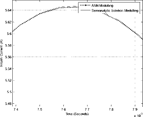
Figure 6: Zooming of first cycle of Inrush current shows difference in ANN1 modeling and semi analytic solution modeling

• b)    Weights between Hidden Layer1 to Hidden

Layer2

		W h1-h2	Hidden Layer1 (Neurons)
v ^	0.11459	2.3128	0.07225	2.0329	0.08479	0.21367
s -^	0.11139	1.3542	0.10149	-3.030	-1.4033	0.16277
	0.34714	7.9291	28.492	5.0615	-7.3575	-40.717

• c)    Weight between Hidden layer-2 to output layer

W h2-o               Input Layer (Neurons)

Output Neuron -9.8719   7.2919     2.219

• d)    Bias Values of hidden layer1

Hidden Layer1 (Neurons)

-1.8686   5.1622   6.3852   -1.3332   1.78   0.22031

• e)    Bias Values of hidden layer2

Hidden Layer2 (Neurons) 1.3763   -0.96866    -5.7563

• f)    Bias Values of Output Layer

  Output Layer (Neurons)     0.41341

Magnetization characteristic is shown in figure 8 using data obtained from semi analytic solution and ANN1. Some part of data for comparison is shown in table-1

Table-1 Comparison of inrush current using semi-analytic and ANN1

S.No	Time	i m	Flux	semi-analytic i inrush	ANN1 i inrush	% Error
1	0.0007	0.2454	0.8509	0.25289	0.2515	-0.5526
2	0.0015	0.3084	0.9425	0.3208	0.3212	0.13072
3	0.005	2.5786	1.8123	2.4908	2.4903	-0.0200
4	0.01	2.9514	1.8678	3.0465	3.0461	-0.0131
5	0.02	0.2792	0.9026	0.30319	0.3036	0.16464
6	0.03	0.1627	0.6899	0.13254	0.1320	-0.3482
7	0.04	1.3891	1.5579	1.3673	1.3667	-0.0439
8	0.05	-0.003	-0.025	-0.0039	-0.002	-36.632

Performance during training of ANN1 with respect to number of epochs is shown by figure 7.

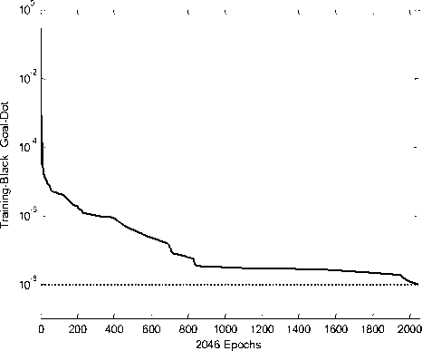
Figure 7: Performance with epochs during training of ANN1 Modeling for inrush current

• B.    ANN2 model for modeling of inrush current’s peak

• 1)    Effect of switching angle

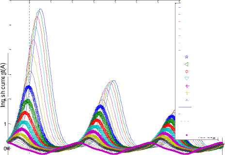
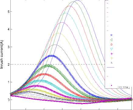
It was observed that switching angle plays a very important role in peak of inrush current as well as time to settle down to no load current value. With zero degree switching, inrush current has highest peak relatively to other switching angles as shown in figure 9. According to this figure 9, highest peak appear with lowest switching angle as well as takes longer time to settle down at no load current value and lowest peak appear with higher switching angle as well as takes lesser time to settle down to no load values. In other words, peak of inrush current and settling time to no load current value, behaves as inversely proportional to switching angle.

Wave form of inrush current with different switching angle is shown in figure 9 and 10 at constant remanent flux i.e. 0.824 Wb. To understand clearly effect of switching angle on peak of inrush current and settling time to no load value is shown by figure 10.

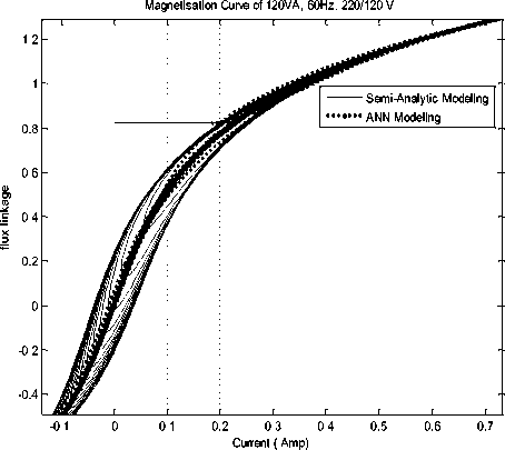
Figure 8: Magnetization curve with ANN1 Modeling (dotted)

Effect of Switching Angle on Inrush Current

0.005    0.01    0.015    0.02   0.025   0.03   0.035    0.04   0.045    0.05

time (sec)

-1

Figure 9: Effects of different switching angle on inrush current with time

0 deg

10 deg

20 deg

30 deg

40 deg

50 deg

60 deg

70 deg

80 deg

90 deg

100 deg

110 deg

120 deg

130 deg

140 deg

150 deg

160 deg

170 deg

180 deg

Effect of Switching Angle on Inrush Current

140 deg

150 deg

160 deg

170 deg

180 deg

-3 x 10^-3

68 time (sec)

Figure 10: Zooming of first cycle with different switching angle of Inrush current with time

0 deg

10 deg

20 deg

30 deg

40 deg

50 deg

60 deg

70 deg

80 deg

90 deg

100 deg

110 deg

120 deg

130 deg

• 2)    Effect of Remanent Flux

Different weights associate with ƒ_ANN2 describes here:

• g)    Weights between Input layer to Hidden Layer-1

  W i-h1	Input Layer (2 Neurons)
  Й	-3.8413 1.2163	4.4941 -3.13
  	1.8156	2.3123
  	-2.1326	-4.6827
  	-0.1166	26.895
  	2.3082	4.199
  	-0.31717	-1.0443
  	3.9155	-6.2348

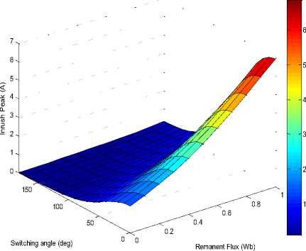
Figure 11: Effect of switching angle and remanent flux on peak of inrush current using semi-analytic solution approach.

• h)    Weights between Hidden Layer1 to HiddenLayer2

  		W h1-h2		Hidden Layer1 (8 Neurons)
  	0.617 64	-0.4 576	0.086	0.42 496	3.10	0.070	0.129	0.51 975
  			948		17	111	57
  р V	0.048	0.27	0.145	-	-	-	-	0.03
  	481	697	96	1.37 78	0.40 96	1.154 4	1.009 5	801
  	2.220 9	0.33 94	4.060 4	1.80 96	0.76 01	1.313 6	3.715 7	0.16 371
  	0.667 77	0.18 03	0.742 12	2.10	3.43 34	1.076 7	0.085 525	0.77 61
  	-	0.50	0.068	-	0.30 40	1.476 7	0.087	0.06
  	1.554	925	421	1.68			242	080
  	-	0.11	0.104 81	0.46	0.19	0.345	0.581	0.00 78
  	1.007	706		918	474	83	9

  
  

• i)    Weight between Hidden layer-2 to output layer

W h2-o                     Hidden Layer2 (6 Neurons)

Output Neuron -4.092   4.9867   0.6031   -3.499   - 2.510   3.138

• j)    Bias Values of hidden layer1

Hidden Layer1 (8 Neurons) 3.9033   -0.110    -4.12   2.299   -16.14   -2.18   -0.34   4.630

• k)    Bias Values of hidden layer2

Hidden Layer2 (Neurons) -3.0764   -1.3229   -0.09180   2.0957   1.1932   1.3745

• l)    Bias Values of Output Layer

Output Layer (Neurons)      2.142

To know accuracy of ANN2 Model, Output data of ANN2 was compared with data which was used to train ANN2 as shown in figure 13.

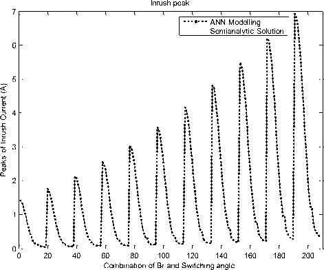
Figure 13: ANN2 Modeling of inrush current’s peak

ANN2 based inrush current’s peak is shown in figure 15. Some part of data is shown in table-2.

2335 Epochs

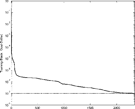
Figure 14: Performance with epochs during training of ANN2 for Inrush current’s peak modeling

Table2. Comparison of Inrush current’s peak prediction using Semi-Analytic and ANN2

S.No.	Br	Switching angle	Semi-Analytic Peak of Inrush Current	ANN2 Based Peak of Inrush	Percentage Error
1	0	0	1.4375	1.4381	-0.04174
2	0	90	0.22458	0.2262	-0.72135
3	0	180	0.049339	0.050723	-2.80508
4	0.1	0	1.7554	1.7554	0
5	0.1	90	0.28484	0.28589	-0.36863
6	0.1	180	0.059083	0.059928	-1.43019
7	0.2	0	2.1266	2.127	-0.01881
8	0.2	90	0.36101	0.36142	-0.11357
9	0.2	180	0.07082	0.071761	-1.32872
10	0.3	0	2.5535	2.5543	-0.03133
11	0.3	90	0.45616	0.45652	-0.07892
12	0.3	180	0.085016	0.086269	-1.47384
13	0.4	0	3.0374	3.0378	-0.01317
14	0.4	90	0.57431	0.57523	-0.16019
15	0.4	180	0.10228	0.10356	-1.25147
16	0.5	0	3.5764	3.5765	-0.0028
17	0.5	90	0.72026	0.72165	-0.19299
18	0.5	180	0.12334	0.12406	-0.58375
19	0.6	0	4.167	4.1673	-0.0072
20	0.6	90	0.89931	0.90051	-0.13344
21	0.6	180	0.14903	0.14878	0.167751
22	0.7	0	4.8041	4.8043	-0.00416
23	0.7	90	1.1171	1.1177	-0.05371
24	0.7	180	0.18035	0.17978	0.316052
25	0.8	0	5.4806	5.4803	0.005474
26	0.8	90	1.3798	1.3798	0
27	0.8	180	0.21817	0.22033	-0.99005
28	0.9	0	6.1879	6.1892	-0.02101
29	0.9	90	1.6929	1.6931	-0.01181
30	0.9	180	0.27554	0.27528	0.09436
31	1	0	6.917	6.9168	0.002891
32	1	90	2.0612	2.062	-0.03881
33	1	180	0.35343	0.35282	0.172594

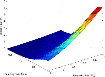
Figure 15: Effect of switching angle and remanent flux on peak of inrush current using ANN2.

• VI. Conclusion

  From the results it is observed that Peak of inrush current and settling time to no load current value is inversely proportional to the switching angle but directly proportional to remanent flux. ANN Model has beauty to train network with data of non-linearity which gives almost exact matching with target values. Therefore ANN1 model gives inrush current value with an average of percentage error of -0.52913 and ANN2 able to predict inrush current’s peak based on remanent flux and switching angle with an average percentage error of -0.00168, which is inacceptable limit. Results of the study suggest thatLM training is faster than the general delta rule and it needs less input pattern to training than the other one.

Performance during training of ANN2 with number of epochs is shown in figure 14. Surface of