Neural network forecasting of time series

By neural networks are meant computational structures that simulate simple biological processes that are somehow related to a person's brain activity. They are parallel systems capable of adaptive learning by analyzing input effects. The elementary converter in these networks is the neuron. Artificial NN are built according to the principles of organization and functioning of their biological analogs. They are able to solve a wide range of problems of image recognition, identification, prediction, optimization, management of complex objects. Special attention should be paid to the use of neural network technologies (dynamic neural networks are the most relevant now) to improve the processing of radar information in difficult conditions, which require high computing power, when the dynamics of changing external conditions are very high and traditional approaches to the creation of processing systems can’t provide the required result [1].

In addition to the ability to solve a new class of problems, neural networks have a number of significant advantages. First, it is resistance to input noise, which allows the use of neural networks in high-precision communication systems. Such an opportunity for neural networks appears due to the so-called training. After training, they are able to ignore the inputs to which noise data is fed. Neural networks are able to function correctly, even if the input is noisy.

Secondly, adaptation to change. This means that with small changes in the environment, the neural network is able to adapt to changes. Consider a neural network that predicts the growth / fall in prices on the exchange. However, gradually, day by day, the situation on the market is changing. If the network did not adapt to these changes, it would stop giving the right answers in a week. But artificial neural networks, learning from the data, each time adjust to the environment. Third, it is fault tolerance. They can give out correct results even at considerable damage of components making them. Fourth, ultra-high speed. The computer executes commands in sequence. However, in the head of a person, each neuron is a small processor (which receives a signal, converts it, and sends it to the output). And there are billions of such processors in our heads. We get a giant network of distributed computations. The signal is processed by neurons simultaneously. This property potentially manifests itself in artificial neural networks. If you have a multi-core computer, this property will be executed. For single-core computers, there will be no noticeable difference [2].

However, neural networks have a serious drawback. It is worth noting that neural networks, despite a wide range of tasks that they can solve, still remain only useful additional functionality. In the first place there are always computer programs. The remarkable news is that by integrating conventional software algorithms and neural networks you can almost completely get rid of all potential flaws.

Studies on artificial neural networks are related to the fact that the way information is processed by the human brain is fundamentally different from the methods used by conventional digital computers. The brain is an extremely complex, nonlinear, parallel computer. He has the ability to organize his structural components, called neurons, so that they can perform specific tasks (such as pattern recognition, sensory processing, motor functions) many times faster than most high-speed modern computers can.

Proceeding from all described above it becomes clear why at this stage of development of methods and methods of programming so much attention is paid to neural network programming [3].

The prediction of time series is currently a topic, as it has a wide field of application (radiolocation, medicine, socio-economic sphere, energy, risk management, engineering applications, etc.). Analysis of works in the field of long-term forecasting (22, 24, 25) of nondeterministic signals showed that at the moment the least studied is neural network long-range forecasting. The use of neural networks for long-term forecasting is based on their ability to approximate non-linear functions, to accumulate history and its application in forecasting and learning ability [4].

Model description

The structure of an artificial neuron can be represented in the form of a model containing three basic elements:

• 1)    A set of synapses characterized by their weights. In particular, the signal x j at the input of the synapse j , connected with the neuron k , is multiplied by the weight w kj ;

• 2)    Totalizer, which adds input signals, weighted relative to the corresponding neuron synapses;

• 3)    The activation function limits the amplitude of the output signal of the neuron [5].

In mathematical terms, the functioning of a neuron is expressed by the following equations (1):

Uk = ^m=iwk:jxj , ук = ф(ик + bk).                                                       (1)

The graphically nonlinear model of a neuron is show in Fig. 1.

The Hecht-Nielsen theorem proves the representability of a function of several variables of a fairly general type by means of a two-layer neural network with direct complete connections to the N compo-

Fig. 1. Nonlinear model of a neuron

nents of the input signal, 2 N + 1 components of the first (“hidden” layer) with previously known limited activation functions (for example, sigmoidal) and M components of the second layer with unknown activation functions. The theorem, therefore, in a non-constructive form proves the solvability of the problem of representing a function of a sufficiently arbitrary form on HC and indicates for each problem the minimum values of the number of network neurons needed for the solution. We show multilayer neural network in Fig 2.

In the study of the neural network, the following formula for estimating the necessary number of synaptic weights Lw in a multilayer (two-layer) network with a sigmoidal activation function was used [6].

^m—— <  L_w <  т Г ^— + 1) (п + т + 1) + т. l+log₂N    ^w      m

Having estimated the necessary number of weights, we can calculate the number of neurons in the hid- den layers. Since a two-layer network was investigated, we will give the formula (3) as applied to it [7].

L =- ^^- . n+m

Having defined a certain network structure, it is necessary to find the optimal values of the weight coefficients. This stage is called teaching the NA. The task of learning is to find (synthesize) some optimal function. It requires long calculations and represents an iterative procedure, the iteration number of which can reach from 10 to 100 000 000 [8]. There are the following basic methods of learning the neural network: local optimization, stochastic optimization, global optimization, training with the teacher, algorithm for back propagation of the error. We chose the algorithm of global optimization, since it is the speedy and less resource-consuming [9]. But this algorithm has its own drawback, it does not allow you to train large dimensions.

The last component of the neural network is the activation function, which, as noted earlier, normalizes the output values and determines the output signal of the neuron as a function of the induced local field [10, 11]. We chose the hyperbolic tangent function (a kind of sigmoidal activation function), which is generally described by expression [12]

Ф , ^V j (n)^ = atanh ^bv j (n)^ , (a, b) >  0.                   (4)

Algorithm of the neural network:

• 1)    I/O coding: neural networks can only work with numbers;

• 2)    Data normalization: the results of the neuro analysis should not depend on the choice of units of measurement;

• 3)    Preprocessing data: removing obvious regularities from the data makes it easier for neural networks to identify nontrivial regularities;

• 4)    Neural network training;

• 5)    Adaptation;

• 6)    Evaluation of the significance of the prediction.

  Fig. 2. Multilayer neural network with sequential connections

  
  

For the study, a two-layer neural network of direct propagation with a sigmoidal activation function and an algorithm for learning the Error Back Propagation was used [13] (Fig. 3).

The number of neural network epochs equal to 175 (the number of views of the training sample) was determined, which is optimal for predicting the strip non-deterministic process. Increasing or decreasing this value can result in retraining or under-training, resulting in chaotic effects in the network (the network will be hypersensitive or vice versa) [14].

The dependence of the exact forecast length on the length of the training sample was studied for a nondeterministic process passed through a bandpass filter with f o = 530 Hz and Δ f = 60 Hz (Fig. 4). We introduce such a condition, the sample is considered accurate if the prediction error is 10% or less.

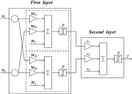
Fig. 3. The model of a two-layer network of direct propagation

In the MATLAB programming environment, a neural network algorithm was implemented [15], a nondeterministic process with a duration longer than the training sequence of the neural network was set up to enable analysis of the accuracy of the forecast.

For the training sequence of the neural network, equal to T o = 3000 samples, we get that the length of the accurately predicted sequence is 17 samples (Fig. 5).

When the length of the training sequence is halved ( T o = 1500 samples), the number of predicted samples is exactly (under given conditions) equal to 14 (Fig. 6).

With the length of the training sequence equal to 750 samples, we obtained an accurately predicted sequence (with errors included) equal to 10 samples. (Fig. 7).

With a training sequence length of 350 samples, an exactly predicted sequence of 6 samples was obtained (Fig. 8).

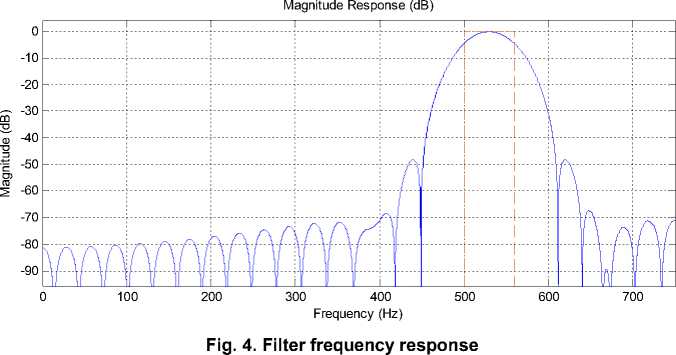
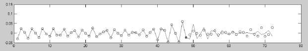
Fig. 5. Band random process and its forecast at T_o = 3000

Fig. 6. Band random process and its forecast at T o = 1500

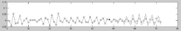
Fig. 7. Band random process and its forecast at T o = 750

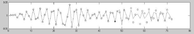
Fig. 8. Band random process and its forecast at T_o = 350

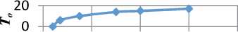
Further reduction of the training sequence does not lead to positive results, the mean square error for the predicted sequence of the first counts exceed 10%, and the predicted sequence become chaotic (Fig. 9). Table 1 show the dependence of the forecast length on the length of the training sample.

Table 1

The dependence of the length of the forecast on the length of the training sample

No.	T o	Т n	T o / Т n
1	3000	17	176,5
2	2000	15	133,3
3	1500	14	107,1
4	750	10	75,0
5	350	6	58,3

О 1ООО 2000 3000 4000

Тп

Fig. 9. Dependence of T_n on T_o

Since the nondeterministic process itself is poorly predicted, it is suggested to use the wavelet transform to increase the length of the exact signal forecast. As a result of this transformation, the original signal is decomposed into several narrowband signals, which are predicted and, by addition, are converted to the original signal. We showed this results on Tables 2 and 3.

Table 2

Dependence of the change in the forecast length on the bandwidth of the signal at T o = 3000

∆ f	т n	∆ f · Т n
1	960	960
10	96	960
20	50	1000
60	16	960
80	13	1040
100	10	1000
120	11	1320
160	11	1760
300	6	1800
400	5	2000
600	4	2400
800	3	2400

Table 3

Dependence of the change in the forecast length on the bandwidth of the signal at T o = 1500

∆ f	т n	∆ f · Т n
1	900	900
10	90	900
20	45	900
60	15	900
80	11	880
100	9	900
120	8	960
160	7	1120
300	5	1500
400	4	1600
600	3	1800
800	2	1600

In Fig. 10 and Fig. 11 shows the Δ f · T n dependence of the bandwidth of a nondeterministic signal. It is seen from the diagram that the dependence has a linear character on three segments. It should also be noted that with increasing spectral processing of the signal up to the Δ f ~ 3 kHz band, the neural network gives an accurate prediction of only one value in advance. From this we can conclude that it becomes a neural network with a short-term forecast.

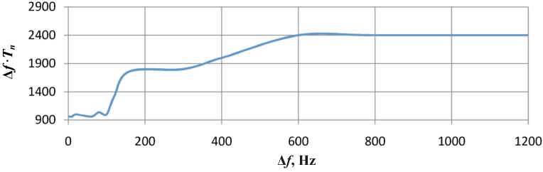
Fig. 10. Dependence Δ f · T n on the signal bandwidth at T o = 3000

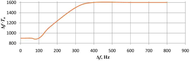
Fig. 11. Dependence Δ f · T_n on the signal bandwidth at T_o = 1500

The dependence of the accuracy of the forecast on the central frequency was studied as follows: from the random sequence, the value of the sine at the central frequency was subtracted, and a prediction of this sequence was provided. Further the forecast developed with the same sinusoid. Thus, the accuracy of the forecast at long-range frequencies was improved.

In the study of this dependence, the following regularity was observed: if the passband of the filter is left unchanged and the center frequency of this band is shifted to the right by Δ f /2, then the accuracy and length of the forecast will remain constant, although the probability of occurrence of “emissions” in the predicted sequence will appear.

The above analysis allows us to choose a rational approach to solving the problem of forecasting nondeterministic processes that are limited in the band, as well as other time series. The choice of this or that method allows to improve the quality of the forecast and its duration. The research was based on the method of neural network prediction using a two-layer network with direct propagation.

Conclusions

Due to the use of realistic radio signals of the neural technology market implemented in a correctly designed, optimized and trained neural network, it was possible to provide a sufficiently high (95–97%) accuracy of the short-term forecast of the listed data.

These results allow us to say that neural network technologies are a powerful tool for solving forecasting problems and allow making forecasts with high accuracy.

Further development of this work is planned in the field of financial, seismology (determining the likelihood of an earthquake) and medicine (determining the probability of occurrence of cardiac diseases by ECG).