New RLS Wiener Smoother for Colored Observation Noise in Linear Discrete-time Stochastic Systems

Published Online December 2013 in MECS DOI: 10.5815/ijitcs.2014.01.02

In comparison with the Kalman estimators, the recursive least-squares (RLS) Wiener estimators have advantages on the point that the RLS Wiener estimators do not require the information of the input noise variance and the input matrix in the state equation. The less information used in the estimators might lead to avoid the degradation of the estimation accuracy instead of using the inaccurate information in the state-space model. In [1], the RLS Wiener filter and fixed-point smoother  are developed  in linear  discrete-time stochastic  systems. The  estimators  require the information of the system matrix, the observation vector, the variance of the state vector in the state equation for the signal and the variance of white observation noise. Also, the Chandrasekhar-type RLS Wiener fixed-point smoother, filter and predictor [2], the square-root RLS

Wiener fixed-point smoother and filter [3] and the RLS Wiener FIR filter [4], etc. are devised in linear discretetime stochastic systems.

Although almost estimators are designed for the white observation noise, there might be actual cases where the observation noise is colored. The estimation problem for the colored observation noise has been treated in the detection and estimation problems for communication systems [5]-[11]. In [9], an alternative method is proposed with regards to the traditional handling of the autoregressive colored observation noise in Kalman filter based speech enhancement algorithm. In [11], based on the autoregressive moving average (ARMA) innovation model, the reduced-order Wiener state estimators are proposed for descriptor system with MA colored observation noise and multiobservation lags.

In [12], the estimation problem of the signal for the white observation noise is considered in linear continuous-time stochastic systems. The spectral factorization method, for the system matrix, the input matrix and the observation matrix, is discussed. Then the innovations state-space model for the colored observation model is developed.

In [13], based on the improved least-squares (ILS) method, the parameter estimation technique is proposed for the signal observed with additional colored noise. In [14], in order to diagnose faults, the optimal state filter is designed for stochastic systems subject to both colored observation noise and unknown inputs.

In [15], starting with the Wiener-Hopf equation, the RLS Wiener fixed-point smoother and filter are presented for the colored observation noise. In [16], with the relation of estimation technique to the innovation theory [17], [18], assuming that the smoothing estimate is given as a linear transformation of the innovation process, the RLS Wiener fixed-interval smoothing algorithm for the colored observation noise, is proposed.

This paper considers on the RLS Wiener estimation problems for the colored observation noise. In the observation equation, the observed value y(k) is given as a sum of the signal z(k) = Hx(k) and the colored observation noise v (k) . In this paper, according to the method in [7], [8], the observation equation is converted to the new observation equation for the white observation noise. In accordance with the observation equation for the white observation noise, this paper proposes new RLS Wiener estimation algorithms for the fixed-point smoothing and filtering estimates in linear discrete-time wide-sense stationary stochastic systems. The RLS Wiener estimators require the following information: (a) the system matrix for the state vector x(k) ; (b) the observation matrix h ; (c) the variance of the state vector x(k) ; (d) the system matrix for the colored observation noise v (k) ; (e) the variance of the colored observation noise.

The remainder of this paper is organized as follows. In section 2, the least-squares fixed-point smoothing problem is introduced for the colored observation noise. In section 3, the RLS Wiener fixed-point smoothing and filtering algorithms are presented. Also, the variance of the innovation process is formulated with regard to the current RLS Wiener filter. In a numerical simulation example of section 4, the estimation characteristics of the proposed RLS Wiener fixed-point smoother and filter are compared with those of [15].

Let the state-space model for x(k) be described as x (k +1) = Фx (k) + Gw( k),

E [ w ( k ) w^T ( s )] = R w ( k)5_K ( k - s ) ,          (4)

where G is an n x l input matrix and _w ( k ) is the white input noise with the auto-covariance function of (4). It is assumed that the stochastic processes of _w (•) and u (•) are mutually uncorrelated.

Let K (•,•) denote the auto-covariance function of v ( k ) . The auto-covariance function K ( k , s ) is given by

K c ( k , s ) =

'A c ( k ) B T ( s ), 0 <  s <  k , _ B c ( s ) A T ( t ), 0 <  k <  s ,

A_c ( k ) = Ф ^k_c , B_C^T ( s ) = Ф - ^sK_c ( s , s ) .

Let the state equation for v ( k ) be given by

II. RLS Wiener Smoothing Problem

Let an m-dimensional observation equation be specified by y (k) = z (k) + vc (k), z (k) = Hx (k)         (1)

in linear discrete-time stochastic systems. Here, H is an m x n observation matrix, z ( k ) is the zero-mean signal vector. The process { v ( k ), k > 0} represents the zero-mean colored observation noise sequence. It is assumed that the signal is uncorrelated with the colored observation noise as

E [ z ( k ) v T ( s )] = 0 , 0 <  k , 5 < да .             (2)

Let K ( k , _s ) = K ( k - _s ) represent the auto-covariance function of the state vector x ( k ) in wide-sense stationary stochastic systems [1], and let K ( k , s ) be expressed in the form of

v c ^{( k +} 1) =^Ф c v c ^{( k} ) ⁺ u ^{( k} ),

E [ u ( k ) u^T ( s )] = R_u ( k)3_K ( k - s ),

in terms of the white input noise vector u ( k ) with the variance R . It is found that, for the expressions

K c ( k + 1, k + 1) = E [ v c ( k + 1) v T ( k + 1)],

K ( k , k ) = E [ v_c ( k ) vj ( k )], in the wide-sense stationary stochastic systems, the following relationships hold.

R u ( k ) = K c ( k + 1, k + 1) -Ф c K c ( k , k ) Ф c , K c ( k + 1, k + 1) = K c ( k , k ) = K c (0)

K x ( k , s )

f A( k ) B T ( s ),

<

[ B ( s ) A^T ( k ),

0 < s < k,0 < k < s,

A ( k ) = Ф ^k , B^T ( s ) = Ф ^{- s}K_x ( s , s ) .

Here, Ф is the transition matrix of _x ( k ) .

In the estimation problem for the colored observation noise, the method of transforming the observation equation into the form of the white observation noise is used [7], [8]. Namely, by introducing

y(k) = y (k + 1)-Ф cy (k), from (1), the following relationship is obtained.

^{y (} k ) = Hx ⁽ k + 1) + v c ⁽ k + 1) ^-Ф c ⁽ Hx ⁽ k ) + v c ⁽ k ))

= ( H Ф-Ф_с H ) x ( k ) + ( HGw ( k ) + u ( k ))        ₍₈₎

= Hx ( k ) + v ( k ),

H = H Ф-Ф_с H , v ( k ) = HGw ( k ) + u ( k ).

Since w ( k ) and u ( k ) are the white noise processes, which are mutually independent, v ( k ) is regarded as the

white observation noise in the transformed observation equation (8).

Based on the transformed observation equation (8) from the observed values y ( k + 1) and y ( k ) , let the fixed-point smoothing estimate x ˆ( k , L ) of x ( k ) be given by

L

x( k , L ) = ^ h ( k , i , L ) У ( i ),                   (9)

i = 1

in terms of the linear transformation of the data { y ( i ), 1 <  i <  L } . Here, h ( k , i , L ) is called the impulse response function.

Let us consider the least-squares estimation problem, which minimizes the mean-square value (MSV)

J = E [|| x ( k ) - x( k , L )||²]                    (10)

of the fixed-point smoothing error. From an orthogonal projection lemma [19],

x ( k ) -£ h ( k , i , L ) y ( i ) 1 y ( 5 ),  1 <  5 <  L ,   (11)

i = 1

the impulse response function satisfies the Wiener-Hopf equation

L

E [ x ( k ) y^T ( 5 )] = ^ h ( k , i , L ) E [ y ( i ) y^T ( 5 )]. (12)

i = 1

Here ‘ 1 ’ denotes the notation of the orthogonality.

The left hand side of (12) is developed as

K ( k , 5 ) = E [ x ( k ) y T ( 5 )]

= E [ x ( k )( Hx ( 5 ) + v ( 5 )) ^T ]

= K_x ( k , 5 ) H^T + E [ x ( k )( HGw ( 5 ) + u ( 5 )) ^T ]   (13)

= K_x ( k , 5 ) H^T + E [ x ( k ) w^T ( 5 )] G^TH^T

= K x ( k , 5 ) H^T + K xw ( k , 5 ) G T H T .

Here, K _w( k , 5 ) = E [ x ( k ) w ^T ( 5 )] represents the crosscovariance function of x ( k ) with w ( s ). Also, the autocovariance function k ( i , ₅ ) = e [ y ( i ) y^T ( ₅ )] is written as

K y ( i , 5 ) = E [( Hx ( i ) + V ( i ))( Hx ( 5 ) + v ( 5 )) ^T ]

= E [( Hx ( i ) + HGw ( i )

+ u ( i ))( Hx ( 5 ) + HGw ( 5 ) + u ( 5 ))) ^T ]           (14)

= HK x ( i , 5 ) H^T + HK xw ( i , 5 ) G^TH^T

+ HGK wx ( i , 5 ) H T

+ (Ru + HGRw (i) GTHT )3k (i - 5), where      the      cross-covariance      function

K wx ( i , 5 ) = E [ w ( i ) x^T ( 5 )] is introduced.

Substitution of (13) and (14) into (12) yields the equation h (k, 5, L) R (5) = K (k, 5) HT

+ K xw ( k , 5 ) G^TH^T

- ]T h ( k , i , L )[ HK x ( i , 5 ) H^T

+ HK xw ( i , 5 ) G^TH^T + HGK wx ( i , 5 ) H^T ],

R (5) = Ru (5 ) + HGRw (5 ) GTHT, which the optimal impulse response function satisfies.

In section 3, by starting with (15), the RLS Wiener estimation equations for the fixed-point smoothing and filtering estimates are derived via the invariant imbedding method.

• III.    RLS Wiener Estimation Algorithms

Under the preliminary assumptions on the linear least-squares estimation problem of the signal z ( k ) in section 2, Theorem 1 presents the RLS Wiener fixed-point smoothing and filtering equations, which use the covariance information of the signal and the colored observation noise.

• Theorem 1

Let the auto-covariance function K ( k , s ) of the state vector x ( k ) be given by (3), let the variance of the colored observation noise v ( k ) be K ( k , k ) , let the variance of the white input noise w ( k ) be R ( k ) and let the variance of u ( k ) in the state equation (6) for the colored observation noise v_c ( k +1) be R _u ( k ). Then, the RLS Wiener algorithms for the fixed-point smoothing and filtering estimates of the signal z ( k ) consist of (16)-(30) in linear discrete-time stochastic systems with the wide-sense stationarities.

Fixed-point smoothing estimate of the signal z ( k ) : z ˆ( k , L )

jB( k , L ) = Hx ( k , L )                          (16)

Fixed-point smoothing estimate of x ( k ) : x ˆ( k , L )

xc(k , L ) = xc(k , L - 1)

+ h ( k , L , L )( y ( L ) - H O< Z j ( L - 1, L - 1)         ⁽¹⁷⁾

• - H Ф c h ₂ ( L - 1, L - 1))

  Smoother gain: h ( k , L , L ) h ( k , L , L ) = ( K x ( k , k )( Φ T ) L - kHT - q ( k , L - 1) Φ THT - q ( k . L - 1) HT ) × [ R ( L ) + H ( Kx ( L , L ) - Φ S 11( L - 1) Φ T -Φ S ( L - 1) Φ T ) HT                 (18) + HGRT ( L ) GT ( Φ T ) - 1 HT - H Φ S ( L - 1) HT - H Φ S ( L - 1) HT ] - 1 Fixed-point smoothing estimate of x ( k ) : x ˆ( k , L ) x ˆ( k , L ) = x ˆ( k , L - 1) + h ( k , L , L )( y ( L ) (19) - H Φ α ˆ ( L - 1, L - 1) -    H Φ α ˆ ( L - 1, L - 1)) q 1 ( k , L ) = q 1 ( k , L - 1) Φ T + h ( k , L , L )( HKx ( L , L ) - H Φ S ( L - 1) Φ T                   (20) - H Φ S 21 ( L - 1) Φ T ), q 1 ( k , k ) = S 11 ( k ) + S 21 ( k ) q ( k , L ) = q ( k , L - 1) Φ T + h ( k , L , L )( HGR w T ( L ) GT - H Φ S ( L - 1) Φ T                  (21) - H Φ S 22 ( L - 1) Φ T ), q ( k , k ) = S ( k ) + S ( k ) Filtering estimate of the signal z ( L ) : z ˆ( L , L ) z ˆ( L , L ) = Hx ˆ( L , L )                       (22) Filtering estimate of x ( L ) : x ˆ( L , L ) x ˆ( L , L ) = Φ x ˆ( L - 1, L - 1) + ( G 1 ( L , L ) + G 2 ( L , L ))( y ( L ) - H Φ x ˆ( L - 1, L - 1)),        ( ) x ˆ(0,0) = 0

  G 1 ( L , L ) = ( K x ( L , L ) HT - Φ S ( L - 1) Φ THT - Φ S 12 ( L - 1) HT ) × [ R ( L ) + H ( K x ( L , L ) - Φ S ( L - 1) Φ T              (24) - Φ S ( L - 1) Φ T ) HT + HGRT ( L ) GT ( Φ T ) - 1 HT - H Φ S ( L - 1) HT - H Φ S ( L - 1) HT ] - 1 G 2 ( L , L ) = ( Φ- 1 GR w GTHT - Φ S ( L - 1) Φ THT - Φ S ( L - 1) HT ) × [ R ( L ) + H ( K x ( L , L ) - Φ S ( L - 1) Φ T           (25) - Φ S ( L - 1) Φ T ) HT + HGRT ( L ) GT ( Φ T ) - 1 HT - H Φ S ( L - 1) HT - H Φ S ( L - 1) HT ] - 1 S 11 ( L ) = Φ S 11 ( L - 1) Φ T + G 1 ( L , L )( HK x ( L , L ) - H Φ S ( L - 1) Φ T          (26) - H Φ S 21 ( L - 1) Φ T ), S 11 (0) = 0 S 12 ( L ) = Φ S 12 ( L - 1) Φ T + G 1 ( L , L )( HGR w T ( L ) GT -    H Φ S ( L - 1) Φ T          (27) - H Φ S 22 ( L - 1) Φ T ), S 12 (0) = 0 S 21 ( L ) = Φ S 21 ( L - 1) Φ T + G 2 ( L , L )( HK x ( L , L ) - H Φ S ( L - 1) Φ T          (28) - H Φ S 21 ( L - 1) Φ T ), S 21 (0) = 0

S₂(LL ) = Ф S₂(LL - 1)Ф^T

+G2( L, L )(HGRw( L) GT

• -    H Ф S(LL - 1) Ф ^T          (29)

• -    H Ф S 22 ( L - 1) Ф ^T ),

S 22 (0) = 0

R ( L) = R u ( L) + HGR w ( L) G^TH^T , R u ( L ) = K c ( L + 1, L + 1) -Ф c K c ( L , L ) Ф ^T _c

= K c (0) -Ф c K c (0) Ф c ,                      (30)

GR w ( L ) G^T = K x ( L + 1, L + 1) -Ф K x ( L , L ) Ф ^T

= K x (0) -Ф K x (0) Ф ^T ,

H = h ф-ф_с h

Proof of Theorem 1 is deferred to the appendix.

From (22) and (23), the variance of the innovation process U(L) = y(L) - HФx(L -1, L -1) is given by

П ( L ) = R ( L ) + H ( K x ( L , L )

• - Ф S J L - 1) Ф ^T

• - Ф S ₂,( L - 1) Ф ^T ) H^T

²¹                                  (31)

+ HGR T ( L ) G^T ( Ф ^T ) ^{- 1} H^T

• -    H Ф S ₂( L - 1) H^T

• -    H Ф S_{2 2}( L - 1) H^T .

• IV.    A Numerical Simulation Example

In this section, to show the efficiency of the estimation characteristics of the proposed RLS Wiener fixed-interval smoother and filter, a numerical example is demonstrated.

Let a scalar observation equation be specified by

y ( k ) = z ( k ) + v_c ( k ) , z ( k ) = Hx ( k ) .       (32)

Here, v ( k ) is the zero-mean colored observation noise. Let the signal z ( k ) be generated by the second-order AR model.

z ( k + 1) = - a_xz ( k ) - a₂z ( k - 1) + w ( k ),

E [ w ( k ) w ( 5 )] = CT 2 5_K ( k - 5 ),              (33)

a_x =- 0.1, a₂ =- 0.8, ct = 0.5.

The corresponding state-space model for z ( k ) can be written as

z ( k ) = Hx ( k ) = x ( k ),   H = [ 1  0 ] ,

Г x , ( k )

x ( k ) =          ,

x 2 ( k )

"x 1 ( k + 1) 1  Г 0     1 IF x 1 ( k ) 1

=                                 (34)

x 2 ( k + 1) J  ^- a2   - ax J^ x ( k )

"0"

+ 1 w ( k ),

E [ w ( k ) w ( 5 )] = R u § K ( k - 5 ).

The auto-covariance function of the signal z ( k ) is given by [15]

K (0) = CT CT

K ( m ) = ст ст {— ^ l i ^ tz ll ^ m--- [( a - a )( aa + 1)]

a ( a ² - 1) a m   .

--}

[( a - a )( aa + 1)]

m >  0,

• a , a = ( - a_x ± ^a 2 - 4 a ₂) / 2.

From (34) and (35), it is found that

K x ( k , k ) =

Ф =

.^{- a} 2

K (0)

K (1)

- a_x

K (1)

K (0)

K (0) = 0.25 , K (1) = 0.125 .

Let the state equation for v (k) be given by vc (k + 1) =Ф cvc (k) + u (k),

E [ u ( k ) u^T ( 5 )] = R_U § K ( k - 5 ),              (37)

Ф c = 0.91,  Ru = 0.01, where u(k) is the white input noise in the state equation (37) for the colored observation noise process. The auto-variance function of the colored observation noise     vc(•)      satisfies     the     relationships

K ( k +1, k +1) = K ( k , k ) = K (0)      and      hence

K (0) = Ru in wide-sense stationary stochastic c      1 - a systems.

Substituting H , ф, K_x ( L , L ) = K (0), ф_с,

K ( L , L ) = K (0) and R_u into the RLS Wiener estimation algorithms of Theorem 1, the fixed-point smoothing and filtering estimates are calculated recursively.

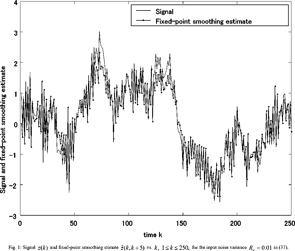
Fig. 1 illustrates the signal z(k) and the fixed-point smoothing stimate Z(k,k + 5) vs. k, 1 < k < 250, for the input noise variance R = 0.01 in (37). Fig. 2 illustrates the MSVs of the filtering errors z(k) - z(k, k) and the fixed-point smoothing errors z (k) - z( k, k + Lag), 1 < Lag < 10, for R = 0.0225, 0.01, 0.0225. The MSVs of the estimation errors by the filtering and fixed-point smoothing algorithms in Theorem 1 are compared with those in the previous estimators [15]. For Lag = 0 , the MSV of the filtering errors z(k) - z(k, k), 1 < k < 2000, is plotted. From Fig. 2, it is indicated that the estimation accuracy of the proposed filter and the fixed-point smoother is superior to that of the estimators in [15]. For R = 0.01,  0.0225,  in comparison with the MSVs of the filtering errors, the MSVs of the fixed-point smoothing errors are improved slightly. As the variances R of the input noise, in the state equation for the colored observation noise, becomes small, the MSVs of the filtering errors and the fixed-point smoothing errors decrease and the estimation accuracy is improved. Here, the MSVs of the fixed-point smoothing and filtering errors are evaluated 2000

by  £(z(k) - z(k,k + Lag)2/2000,  1 < Lag < 10, and k=1

у ( z ( k ) - z( k , k )) 2 /2000..

k = 1

<п

а> ио

Е

<л

л ею

> > 00

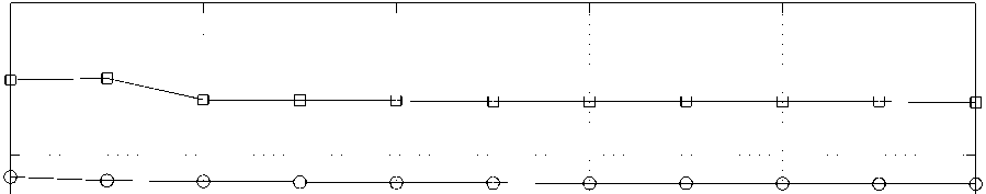
Fig. 2: MSVs of the filtering errors z ( k ) - z(k , k ) and the fixed-point smoothing errors z ( k ) — z ( k , k + Lag ), 1 <  Lag < 10, for

R = 0.0225,  0.01,  0.0225. .

• V.    Conclusions

In this paper, the RLS Wiener filter and the fixed-point smoother have been designed for the colored observation noise. In particular, the observation equation (1) is converted to the new observation equation      (8)      by     the      transformation

y ( k ) = y ( k +1) — Ф_с y ( k ). By this transformation, the observation equation (1) for y ( k ) with the additive colored observation noise v ( k ) is converted to (8) for y ( k ) with the additive white observation noise v ( k ) .

A numerical simulation example has shown that the proposed RLS Wiener algorithms for the fixed-point smoothing and filtering estimates are feasible. From Fig. 2, it is indicated that the estimation accuracy of the proposed filter and the fixed-point smoother is superior to that of the estimators in [15]. For R = 0.01,  0.0225, in comparison with the MSVs of the filtering errors, the MSVs of the fixed-point smoothing errors are improved slightly.

As in [15], [16], the RLS Wiener estimators do not require the information of the input noise variance Q ( k ) and the input matrix G in the state equation (4), in comparison with the Kalman estimation technique [19]. In the RLS Wiener estimators, we are not anxious about the degradation in the estimation accuracy caused by the modeling errors for Q ( k ) and G .