Non-isothermal Flow through a Curved Channel with Strong Curvature

Published Online August 2013 in MECS

• I.    Introduction

  The study of flows and heat transfer through curved ducts and channels has been and continues to be an area of paramount interest of many researchers because of the diversity of their practical applications in fluids engineering, such as in fluid transportation, turbo machinery, refrigeration, air conditioning systems, heat exchangers, ventilators, centrifugal pumps, internal combustion engines and blade-to-blade passage for cooling system in modern gas turbines. Blood flow in the human and other animals also represents an important application of this subject because of the curvature of many blood vessels, particularly the aorta. The flow through curved a duct shows physically interesting features under the action of centrifugal force caused by the curvature of the duct. The presence of curvature produces centrifugal forces which acts at right angle to the main flow direction and creates secondary flows. Dean (1927) was the first who

  formulated the problem in mathematical terms under the fully developed flow conditions and showed the existence of a pair of counter rotating vortices in a curved pipe. In consideration of the importance, flows in curved ducts have been studied extensively in the literature for several decades, the readers are referred to Berger et al . (1983), Nandakumar and Masliyah (1986), Ito (1987) and Yanase et al. (2002) for some outstanding reviews on curved duct flows.

The non-linear nature of the Navier-Stokes equation, the existence of multiple solutions does not come as a surprise. The solution structure of fully developed flow is commonly present in a bifurcation diagram which consists of a number of lines (branches) connecting different possible solutions. These branches can bifurcate and show multiple solutions in limit points (Mondal, 2006). An early complete bifurcation study of two-dimensional (2-D) flow through a curved duct of square cross section was conducted by Winters (1987). Very recently, Mondal et al . (2007a) performed comprehensive numerical study on fully developed bifurcation structure and stability of two-dimensional (2D) flow through a curved duct with square cross section and found a close relationship between the unsteady solutions and the bifurcation diagram of steady solutions. The flow through a curved duct with differentially heated vertical sidewalls has another aspect because secondary flows promote fluid mixing and heat transfer in the fluid (Yanase et al ., 2005). They also studied the transitional behavior of the unsteady solutions by time evolution calculations.

Many researchers have performed experimental and numerical investigation on developing and fully developed curved duct flows. An early complete bifurcation study of two-dimensional (2-D) flow through a curved duct with square cross section was performed by Winters (1987). Our ultimate goal is to investigate the non-isothermal flows through a curved channel with the presence of buoyancy effects by considering the strong curvature. Mondal et al. (2006) performed numerical prediction of non-isothermal flow through a curved square duct over a wide range of the curvature and the Dean number. They showed that stability characteristics drastically change due to an increase of curvature. However, there has not yet been done any substantial work regarding the flow characteristics through a curved square duct for large curvature ; this paper is, therefore, an attempt to fill up this gap with the investigation of the flow characteristics through a curved square channel for strong curvature because this type of flow is often encountered in engineering applications. From the scientific as well as engineering point of view, it is quite interesting to study curved channel flows with differentially heated vertical sidewalls for the large Grashof number, because this type of flow is often encountered in engineering applications. The present study is, therefore, an attempt to fill up this gap with the study of the non-linear behavior of the unsteady solutions by time-evolution calculation.

In the present paper, a numerical study is presented for the fully developed two-dimensional flow of viscous incompressible fluid through a curved square channel with differentially heated vertical sidewalls. Flow characteristics are studied over a wide range of the Dean number and the strong curvature by finding the steady solutions, investigating their linear stability and analyzing nonlinear behavior of the unsteady solutions by time evolution calculations.

• II.    Governing Equations

Consider a hydro dynamically and thermally fully developed two-dimensional flow of viscous incompressible fluid through a curved duct with square cross section. Let 2 d be the width of the cross section. The coordinate system with the relevant notations is shown in Fig 1. Where C is the centre of the curvature and L is the radius of the curvature. Let x and y axes are taken to be in the horizontal and vertical directions respectively, and z is the coordinate along the centerline of the duct, i.e., the axial direction. It is assumed that the outer wall of the duct is heated while the inner one is cooled. The temperature of the outer wall is T ₀ + A T and that of the inner wall is T ₀ - A T , where A T > 0.

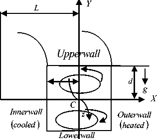
Fig. 1: Coordinate system of the curved square duct

It is also assumed that the flow is uniform in the axial direction, and that it is driven by a constant f      dP')

pressure gradient G I G =-- I along the center-line

(       d z ')

of the duct. The main flow in the z direction as in Fig. 1.

The dimensional variables are then non-dimensional zed by using the representative length l , the representative velocity Uo = — , where и is the

0d kinematic viscosity of the fluid. We introduce the non-dimensional variables defined as

u = u' U0, v v'        V25  , = —, w =---w U0      Uo x = x/ d, - y      z y=1 ’   z=d T T' , AT' t = U0 t',   5 = d, d ,         L, P P ‘ гг_  дP'  d PU 02 д z' pU,2 where u,v and w are the non-dimensional velocity components in the x, y and z directions, respectively; t is the non-dimensional time, P is the non-dimensional pressure, 5 is the non-dimensional curvature defined as 5 = —, and temperature is non- dimensional zed by AT . Hence forth, all the variables are non-dimensional zed if not specified.

Since the flow field is uniform in the z direction, the sectional stream function / is introduced as

1 д/         1 д/ u =--, V =---

A new coordinate variable y is introduced in the y h direction asy = ay , where a = — is the aspect ratio of the duct cross section. In this study, we consider the case for h = l i.e. a = 1 (square duct). Then, the basic equations for w, / and T are expressed in terms of non-dimensional variables as

⁽ 1 ^{+ 5} x ⁺ д t

^ w / ) - Dn + A wL d ( x , y )         1 + 5 x

(1 + 5 x ) A 2 w -

--w + 5—

1 + 5 x д y        д x

и 5 д \ду а 21^

(    1 + 5 x д x ) д t

1     д ( А 2 ^ , ^ )

(1 + 5 x )   д ( x , у )

ду

+--у

(1 + 5 x )²

^д У (

2А₂ у -

3 5 д у д ² у

д x ²

_-

ду д2у д x дx ду

+-------тх

(1 + 5 x )²

д ² у   3 5 ² ду

35 —----- д x2  1 + 5 x д x

2 5 д _л ---А ₂ у

• 1    + 5 x д x д w + w—

• 2             ат

+А₂ ² у - Gr (1 + 5 x ) — д x

д Т      1     д ( Т , у )

д t (1 + 5 x ) д ( x , у )

Pr ^ ²    1 + 5 x д x _v

where,

₌ д² д²

²   д x ²   д у ²,

д(Т,у) s дf дд_дф дд д(x, у)   дx ду  ду дx

The non-dimensional parameters Dn , the Dean number, Gr , the Grashof number, andPr, the prandtl number, which appear in equation (2) - (4) are defined as

Gd ³  2 d

Dn =--J— ци у L

Gr = и

Pr = -к

Where ц , в , к and g are the viscosity, the coefficient of thermal expansion, the co-efficient of thermal diffusivity and the gravitational acceleration respectively is the viscosity of the fluid. In the present study, only Dn is varied while 5 , Gr and Pr are fixed as 5 = 0.5 , Gr = 100 and Pr = 7.0 (water). The rigid boundary conditions used here for w and у are

w ( ± 1, у ) = w ( x , ± 1) = y ( ± 1, у ) = y ( x , ± 1)

= У ( ± 1, у ) = | ^У ( x , ± 1) = 0

д x          д у                          (7)

and the temperature T is assumed to be constant on the walls as

Т (1, у ) = 1, Т ( - 1, у ) =- 1, Т ( x , ± 1) = x

у ^- у w (x, у, t) ^ w (x, - у, t), у( x, у, t) ^-у( x, - у, t), Т (x, у, t) о-Т (x, - у, t)

Therefore, the case of heating the inner sidewall and cooling the outer sidewall can be deduced directly from the results obtained in this study. Equations (2) – (4) would serve as the basic governing equations which will be solved numerically as discussed in the following section.

III. Numerical Calculations

The present study is based on numerical calculations to solve the equation (2)-(4), the spectral method is used. This is the method which is thought to be the best numerical method for solving the Navier-Stokes as well as energy equations (Gottlieb and Orszag, 1997). By this method the variables are expanded in a series of functions consisting of Chebyshev polynomials. The expansion functions ф ( x ) and у ( x ) are expressed as

ф п ( x ) = (1 - x ² ) C n ( x ), У п ( x ) = (1 - x ² ) ² C n ( x )

where C n ( x ) = cos ( n cos 1 ( x ) ) is the n th order Chebyshev polynomial.    w ( x , у , t ), y ( x , у , t )   and

T ( x , y , t ) are expanded in terms of the expansion

functions ф ( x ) and y_n ( x ) as:

,   . MN ^wmn ⁽ t ^{) x}

w ⁽ x , у , t ) = XX       . .    . .

m = 0 n = 0   У т ( x ) y n ( у )

,   . MN ^y mn ⁽ t ) ^x

y(x,у,t) = XX       z     z , m=0n=0  Ут (x)yn (у)

M N Tmn

х

Т ( x ,, у , t ) = XX m = 0 n = 0 y m ( x ) y _n ( у )

where M and N are the truncation numbers in the x and y directions respectively .

The collocation points (x , y ) are taken to be xi = cos

i

M + 2

y = cos

j )

N + 2 J

i = 1, . , M + 1

		^     (12)
j = 1, .	., N + 1

The approximate solution of Eq. (14), thus evaluated, is a function of A t as well as x and t , and the true solution is the limit of the approximate one as A t ^ 0 . The method, determined by Eq. (15), is called the Crank-Nicolson method. The Adams-Bashforth Method, on the other hand, is used for numerically solving initial value problems for ordinary differential equations. This method is an explicit linear multistep method that depends on multistep previous solution points to generate a new approximate solution point.

where i = 1, . , M +1 and j = 1, . , N +1 . Steady solutions are obtained by the Newton-Rapshon iteration method assuming that all the variables are time independent. The convergence is assured by taking sufficiently small £ _p ( £ _p < 10 ¹⁰ ) defined as

MN

£p =IS m =0 n=0

L^{( p +1)}_ _w ^p )²₊L( ^{p +1)}_)²

\ mn     mna J ' \ mmn     т mn)

.  (13)

Дт ^{( p +1)} _ ^pp У mn     mn

The present numerical calculation, for sufficiently accuracy of the solutions, we take M = 20 and N = 20 for a square duct. Finally, in order to calculate the unsteady solutions, the Crank-Nicolson and Adams-Bashforth methods together with the function expansion (11) and the collocation methods are applied to equations (2)-(4).

• IV.    Time-evolution Calculation

In order to solve the non-linear time evolution equations, we use the Crank-Nicolson and Adams-Bashforth method. For the Crank-Nicolson method more explicitly, we consider the following onedimensional heat-flow equation dq    5 2 q dt     dx 2

• V.    Results and Discussion

  In this study, we have investigated time evolution of the resistance coefficients X for the non-isothermal flows through a curved square channel with strong curvature 6 = 0.5 . We have studied the steady and unsteady solutions of the flows at various Dean numbers, Dn 100 <  Dn <  6000 for a fixed Grashof ^,

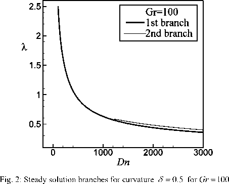
• 5.1    Steady Solution

  With the present numerical calculation, we obtain two branches of steady solutions for Gr = 100 over the Dean number 0 <  Dn <  3000 by using the path continuation technique as discussed in Keller (1987). The two steady solution branches are named the first steady solution branch (first branch, bold solid line) and the second steady solution branch (second branch, thin solid line), respectively. Fig. 2 shows solution structure of the steady solutions for the flow through a curved square channel with strong curvature . It is found that there exists no bifurcating relationship between the two branches of steady solutions as shown in Fig. 2. In the following, the two steady solution branches as well as the flow patterns and temperature profiles on the respective branches are discussed.

number Gr = 100 . In addition to the time evaluation of X , the secondary flow patterns, axial flow distributions and temperature profiles at various Dean numbers are discussed in detail.

where q ( t ) the temperature is at time t regarded as a function of x and T is the heat conductivity. The first time derivative in Esq. (14) is replaced by a finite difference ratio and a time step A t , the derivative with respect to time may be written as

8 q ^ q ( t + ^A t ) - q ( t ) as a t ^ 0

d t         A t

Now taking the average at t and t + 1 , Esq. (14) becomes approximately,

q ( t + A t ) - q ( t ) _ t 5 ²

A t

2 5 x ²

[ q ( t + A t ) - q ( t )]       (15)

• 5.2    Unsteady Solutions:

0.49 0.42 0.35 0.28 0.21

Time evolution of the unsteady solutions for Dn < 4345

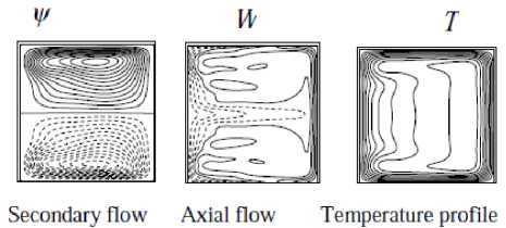
We performed time evolution of the resistance coefficient X for Dn <  4345 at Gr = 100 , and it is found that the flow is steady-state for all the values of Dn in this range. Fig. 3(a) shows time evolution of X for Dn = 4345 . Typical contours of secondary flow, axial flow distribution and temperature profiles for at Dn = 4345 are shown in the Fig. 3(b). As seen in Fig. 3(b), the secondary flow is two-vortex solutions for the steady-state solution. If the Dean number is increased a little for example Dn = 4350, the steady flow turns into periodic solution. It is found that the transition from steady-state solution to periodic oscillation occurs for 5 = 0.5 between Dn = 4345 and Dn = 4350.

Dn=4345

Gr=100

Timeft)

(a)

(b)

Fig. 3: (a) Time evolution of X for Dn = 4345 and Gr = 100 at time 20 <  t <  40 for the large curvature 5 = 0.5 ; (b) Contours of secondary flow, axial flow distribution and temperature profile for Dn = 4345 at time t = 25

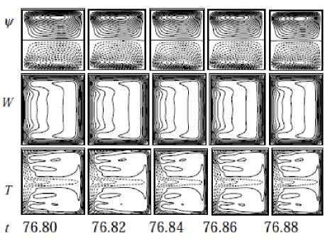
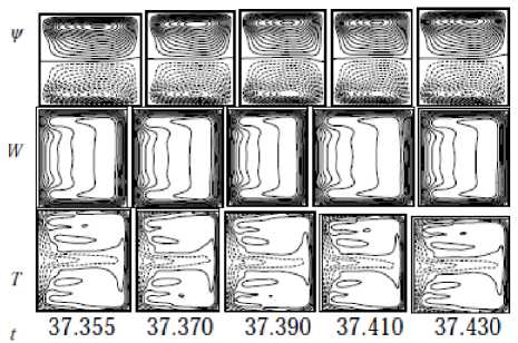
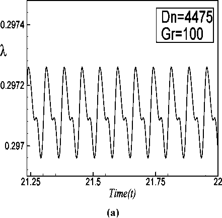
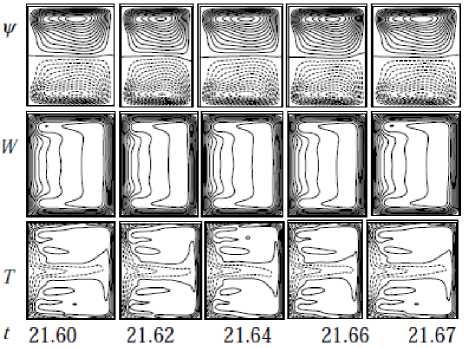
fundamental frequency and its harmonics are seen, which suggests that the flow is periodic for both the cases. Typical contours of secondary flow; axial flow distribution and temperature profiles are shown in Fig. 4(c) for Dn = 4350 and in Fig. 5(c) for Dn = 4440 for one period of oscillation at time 76.80 <  t <  76.88 and 37.355 <  t < 37.430 As seen in Fig. 4(c) and 5(c), the secondary flow is a two -vortex solutions for both Dn = 4350 and Dn = 4440. Next we investigate time evolution of X for Dn = 4475 as shown in Fig. 6(a). It is found that the flow oscillates multi-periodically. Then to justify whether the flow is periodic or multiperiodic, we plot the power spectrum of the time change of X at Dn = 4475 in Fig. 6(b), where it is seen that only the line spectrum of the fundamental frequency and its harmonic are available but no other line spectrum with smaller frequencies are seen, which suggests that the flow is periodic but not multi-periodic. Then typical contours of secondary flow patterns; axial flow distribution and temperature profiles are shown in Fig. 6(c) for Dn = 4475 , one period of oscillation at time 21.60 <  t <  21.67 As seen in Fig. 6(c), the secondary flow is two -vortex solution for Dn = 4475 . Thus it is seen that the periodic oscillations from Dn = 4350 to Dn = 4475 oscillates between two-vortex solution. If the Dean number is increased further, for example Dn = 5050 , the flow turns into multiperiodic. Thus the transition from periodic to multiperiodic oscillation occurs between Dn = 4475 and Dn = 4500

0.3016

X

Dn=4350

Gr=100

(a)

0.0006

Dn=4350 Gr=100

Time evolution of the unsteady solutions for 4350 <  Dn <  4475

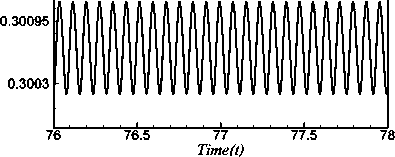
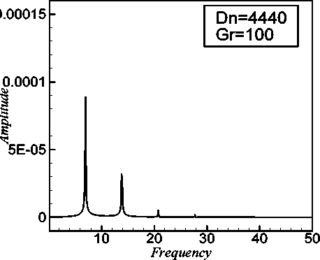
We studied the time evolution of the resistance coefficient X for 4350 <  Dn <  4440 . It is found that the flow is periodic for all the values of Dn in the above range. Fig. 4(a) and Fig. 5(a) show that the flow is periodic oscillations for Dn = 4350 and Dn = 4440. In order to investigate the periodic behavior more clearly, power spectrum of the time evaluation for Dn = 4350 and Dn = 4440 are shown in Fig. 4(b) and 5(b) respectively, where the line spectra of the

0.0004

II

"^0.0002

20     30     40

Frequency

(b)

(с)

(c)

Fig. 4: (a) Time evolution of X for Dn = 4350 at time 76 <  t <  78 for 6 = 0.5; (b) Power spectra of the time evolution of X for

Dn = 4350 for 6 = 0.5 ; (c) Contours of secondary flow, axial flow distribution and temperature profiles for Dn = 4350 at time 76.80 <  t <  76.88

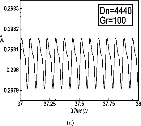
Fig. 5: (a) Time evolution of X for Dn = 4440 at time 37 <  t <  3 8 for 6 = 0.5 ; (b) Power spectra of the time evolution of X for

Dn = 4440 for 6 = 0.5; (c) Contours of secondary flow, axial flow distribution and temperature profiles for Dn = 4440 at time 37.355 <  t <  37.430

0.0004 -

1^о.ооог -

о -о

(b)

Dn=4475Gr=100

5      10     15     20     25

Frequency

(b)

(a)

(c)

Fig. 6: (a) Time evolution of X for Dn = 4475 at time 21.25 <  t <  22 for 5 = 0.5 ; (b) Power spectra of the time evolution of X for Dn = 4475 for 5 = 0.5 ; (c) Contours of secondary flow, axial flow distribution and temperature profiles for Dn = 4475 at time 21.60 <  t <  21.67

Time evolution of the unsteady solutions for 4500 <  Dn <  5050

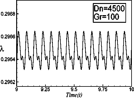
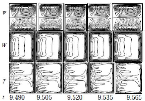
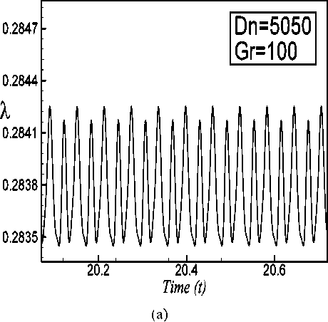
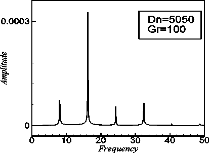
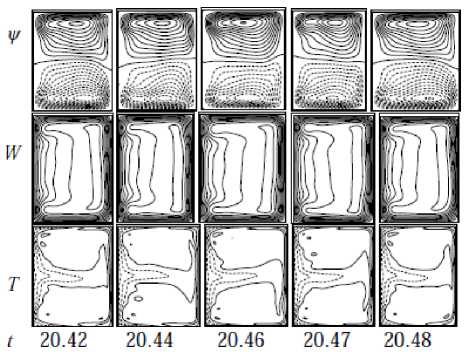
Next we investigate time evolution of for 4500 <  Dn <  5050. It is found that the flow oscillates multi-periodically for 4500 <  Dn <  5050. Fig. 7(a) and 8(a) show the instance of multi-periodic oscillation for Dn = 4500 and Dn = 5050 respectively. In order to investigate the multi-periodic behavior more clearly, power spectrum of the time evaluation of for Dn = 5050 is shown in Fig. 8(b), in which not only the line spectrum of the fundamental frequency and its harmonics but also other line spectrum and its harmonics are seen, which clearly suggests that the flow is multi-periodic. To observe that the change of the flow characteristics contours of typical secondary flow patterns, axial distribution and temperature profiles are shown in Fig. 7(b) for Dn = 4500 and in Fig. 8(c) for Dn = 5050 shown that one period of oscillation at time 9.490 <  t <  9.565 and 20.42 <  t <  20.48 respectively. As seen in Fig. 7(b) and 8(c), the secondary flow two-vortex solutions are found for both Dn = 4500 and Dn = 5050. If the Dean number is increased further, for example Dn = 5075 , the flow turns into chaotic. It is found that the transition from multi-periodic to chaotic oscillation occurs between Dn = 5050 and Dn = 5075

(b)

Fig. 7: (a) Time evolution of X for Dn = 4500 at time

9 <  t <  10 for 5 = 0.5 ; (b) Contours of secondary flow, axial flow distribution and temperature profiles for Dn = 4500 at time

9.490 <  t <  9.565

(b)

Dn = 5075 and one period of oscillation at time 45.00 <  t <  45.40, and for Dn = 5835 one period of oscillation at time 20.00 <  t <  20.40 in Fig. 10(c). If the Dean number is increased further, for example Dn = 5840, the flow turns into periodic. The transition from chaotic to periodic oscillation occurs between Dn = 5835 and Dn = 5840

0.296

0.292 - X

Dn=5075Gr=100

(c)

Fig. 8: (a) Time evolution of X for Dn = 5050 at time

20.08 < t < 20.72 for 5 = 0.5 ; (b) Power spectra of the time evolution of X for Dn = 5050 for 5 = 0.5 ; (c) Contours of secondary flow, axial flow distribution and temperature profiles for Dn = 5050 at time 20.42 < t < 20.48

0.288

0.284

0.28

Time(t)

(a)

(b)

Time evolution of the unsteady solutions for 5075 <  Dn <  5835

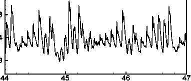
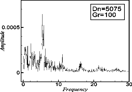
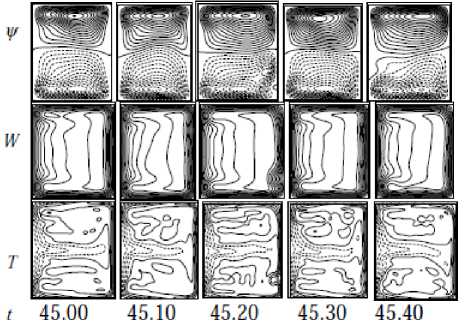
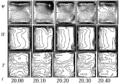
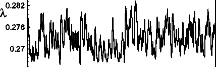
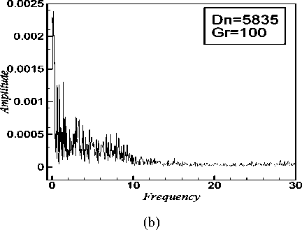
We perform time evolution of for 5075 <  Dn <  5835 . It is found that all the flow oscillates irregularly that is the flow is chaotic in this range. Fig. 9(a) and Fig. 10(a) show the instances of chaotic oscillations for Dn = 5075 and Dn = 5835 respectively. In order to investigate the chaotic behavior more clearly, power spectra of the time evaluation of X for Dn = 5075 and Dn = 5835 are shown in Fig. 9(b) and 10b) respectively. To observe that the change of the flow characteristics, contours of typical secondary flow patterns, axial distribution and temperature profiles are shown in Figure 9(c) and Fig. 10(c) for Dn = 5075 and Dn = 5835 respectively, where it is seen that the chaotic oscillation for Dn = 5075 and Dn = 5835 oscillates between asymmetric two-vortex solutions. Contours of secondary flow patterns, axial distribution and temperature profiles are shown in Fig. 9(c) for

(c)

Fig. 9: (a) Time evolution of X for Dn = 5075 at time 44 <  t <  47 for 5 = 0.5 ; (b) Power spectra of the time evolution of X for

Dn = 5075 for 5 = 0.5 ; (c) Contours of secondary flow, axial flow distribution and temperature profiles for Dn = 5075 at time 45.00 <  t <  45.40

(c)

Fig. 10: (a) Time evolution of X for Dn = 5835 at time 16.10 <  t <  21 for S = 0.5 ; (b) Power spectra of the time evolution of X for Dn = 5835 for S = 0.5 ; (c) Contours of secondary flow, axial flow distribution and temperature profiles for Dn = 5835 at time 20.00 <  t <  20.40

0.294

Dn=5835Gr=100

0.288

0.264

17        18        19       20       21

Time(t)

(a)

number Dn ,100 <  Dn <  6000 and the Grashof number Gr = 100 for the curvature S = 0.5. After a comprehensive survey over range of the parameters two branches of asymmetric steady solutions are obtained for Dn lying in the range. Contours of typical secondary flow patterns, axial flow distribution and temperature profiles are also obtained at several values of the Dean number for the steady-state, periodic, multi-periodic and chaotic solutions.

For the unsteady solution we obtain two-, three- and four-vortex solutions. Then, in order to investigate the non-linear behavior of the unsteady solutions, time evaluations calculations as well as their spectral analysis are performed. It is found that the flow becomes steady-state for Dn <  4345 periodic for 4350 ≤ ≤ 4475 , multi-periodic solutions for 4500 ≤ ≤ 5050 , and chaotic solutions for 5075≤ ≤ 5835. Thus the unsteady flow undergoes in the scenario “ steady ^ periodic ^ multi-periodic ^ chaotic ”, if Dn is increased up to 5835, i.e. Dn <  5835 . If the Dean number is increased further, that is, Dn >  5840 the unsteady flow undergoes through various flow instabilities, if Dn is increased gradually. Thus, in order to investigate the transition from periodic to multi-periodic oscillation or the multiperiodic oscillation to chaotic state in more detail, the spectral analysis is found to be very useful. So, the transition of the unsteady solutions is clearly determined by the power spectrum of the solution.

• VI. Conclusions

In this present study, a detailed numerical study on the fully developed two-dimensional flow of viscous incompressible fluid through a curved channel with strong curvature has been performed by using the spectral method and covering a wide range of the Dean