Non-parametric algorithms of reconstruction of mutually ambiguous functions from observations

Introduction. The problem of function reconstruction from observations when the studied process is described by mutually ambiguous characteristics is considered. This task comes to a problem of approximation, the main feature of which is the lack of aprior information about a parametrical structure of the studied process model. Nonparametric estimation of mutually ambiguous characteristics, some modification and results of numerical studies are offered.

At reconstruction of regression functions from observations nonparametric estimates are often used. At the same time it is supposed that the nature of its dependence is unambiguous on an argument. Hereafter, the problem of function reconstruction from observations at mutually ambiguous dependence is considered. This demanded the introductoin of some changes into the known estimation of Nadaraya-Watson [1].

Aprior information. Aprior information – a set of known in advance data of the studied process, criteria of optimality and restrictions. The criterion of optimality expresses those requirements which have to be best satisfied and restrictions define our opportunities. Thus, the aprior information known to the researcher at an initial stage is a basis for a mathematical formulation of the task [2]. And in essence substantially predetermines a research method [3].

In various computer systems of modelling an important role belongs to reconstruction of functions from observations, in particular to mutually ambiguous function which can be applied at creation of, for example, robots, robotic systems moving on in an unknown area (the area with an unknown terrain).

The levels of aprior information are important during the modelling and control of discrete continuous process-ses. The processes proceeding continuously in time but the variables of which are controlled at discrete time points are related to such processes. Let us point out the following levels of aprior information [4]:

• 1.    Systems with full information. In this case an operator of the process is exactly known, and the casual disturbances affecting an object and connection channels are absent. During the solution of identification and control problems, the methods of mathematical theory of optimum processes and also other methods of synthesis and analysis of control systems can be used.

• 2.    Systems with incomplete information. These are systems with independent (passive) accumulation of information. In this case, the effect of input influence is perceived as simply random influence. Disrurbances are usually assumed in the theory of stochastic systems as

• 3.    Systems with active accumulation of information. The characteristic of these systems is that problems of identification and the task of control can be integrated because sample units of measurements consistently come to the training model and a control system. Thus in case of association of these tasks, the elaboration of control impacts has ambivalent (dual) character – they have to be both exploring and controlling [2; 3]. However if the disturbances operating the process are additive in channels of measurement as well, then in general the system of dual control can become open, its rate of information accumulation does not depend on values of input variables. Such systems are called leading to open or neutral. But there exists a class of non-neutral systems, i. e. a class of irreducible systems.

• 4.    Systems with parametric ideterminacy. A parametric level of aprior information assumes the existence of a model parametrical structure and some characteristics of random disturbances, such as zero mathematical expectation and limited dispersion which are usual. For estimation of parameters various iterative probabilistic procedures are used more often. Under these conditions the problem of identification in narrow sense, as well as in all previous cases, is also solved.

• 5.    Systems with nonparametric uncertainty. A nonparametric level of aprior information does not assume the existence of a model but demands the existence of some data of qualitative character about the process, for example, unambiguity or ambiguity of its characteristics, linearity (for dynamic processes) or the nature of its nonlinearity. Methods of nonparametric statistics are applied to the problem of identification at this level of aprior information solving (identification in a broad sense [5]).

• 6.    Systems with parametric and nonparametric uncertainty. From the point of view of practice, the tasks of identification of multivariable systems under conditions when the volume of initial information does not correspond to any of the above described levels are important. For example, for separate characteristics of a multivariable

random impact on an object. Besides, the class of operators is not known exactly but the assumptions of density of distribution of all random factors are necessary. The density of probability of random factors affecting an object and in channels of variables measurement are usually assumed normal and additive. It is clear that in this case the existence of selection of input and output variables of an object is necessary and observations are statistically independent. Systems with incomplete information are related to the class of open or neutral systems.

process on the basis of physical-chemical and energy regularities, a law of conservation of mass, balance ratios parametrical regularities can be deduced, but for others can not be deduced. Thus, we are in the situation when the task of identification is formulated under conditions of both parametric and nonparametric aprior information. Then models represent the interdependent system of parametric and nonparametric ratios.

Nonparametric approach. Nonparametric estimates of probability density of p ( x ) from observations x i , i = 1, 5 are the basis of this approach. Nonparametric estimates of multidimensional probability density were considered in [1; 6] in details and are given as:

5 к < j _ „j A ps (x)=- Z - П ф —-       (1)

• ⁵ i - 1 ^C5 j = 1 I ^C5    J

where P_s ( x ) – estimation of density of elements distribution; s – sample size; k – a vector lenth x.

Here Ф( v ) – a kernel – the finite bell-shaped function integrating with a square which satisfies the conditions [1; 4; 6]:

0 <  Ф( V ) <« V v eo ( v ), Z [Ф I ^{x x}i J dx = 1,

^C5^J I ^C5 J

The blurring parameter c_s meets the following conditions:

• ^C5 >  0, lim 5 ^„ ^{5 (} c 5 ) k = ^ , lim 5^ c_s = 0 . ⁽⁴⁾

Nonparametric estimation of regression function from observations. For reconstruction of function of regression of M{y|x} from observations {xi,yi, i = 1,5 } we use nonparametric estimates of density of probability (1). As, M{y|x} looks as follows:

I yp ⁽ x , y ) dy

M{ y | x } = ^{n (} y )                          (5)

J p ( x , y ) dy

Q ( y )

Replacing in (5) p ( x , y ) by nonparametric estimates (1) and using property:

.1 J y Ф I y_yi_ I dy = y , i = 1, 5 ,          (6)

^C5 П ( y )     V ^C5    )

it is easy to receive nonparametric estimation of function of Nadaraya–Watson regression which for a onedimensional case looks as follows:

lim n ^»

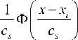
= 5 ( x ^- xi) ,

where c s – a blurring parameter defining the size of the carrier and “delta-shape” of a kernel Ф( v ) [4].

In a computing experiment the bell-shaped functions

Ф( v ) of different types are used, for example:

[ 0.5, v | <  1, Rectangular kernel: Ф( v ) = [

[ 0,     v >  1.

[ 1 - | v |, | v | <  1,

Triangular kernel: Ф( v ) = [                         (3)

[ 0,        |v | >  1.

Y 5 ( x ) =

s

Z у.ф i=1

s

Z Ф i=1

x

^- xi

cs

^- x i

s

and for a case if x a k -dimensional vector it is equal:

Y 5 ( x ) =

sk

Z y i П Ф i = 1 j = 1

Parabolic kernel: Ф( v ) =

[ 0.75(1 - v ) 2 , | ^v | < ¹ [ 0,                |v | >  1.

sk zn Ф i=1 j=1

In fig. 1, 2 function Ф( x/c s )/ c s constructed for three values of a blurring parameter c s = 0.2, 0.4, 0.6. is presented.

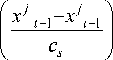
where x i , y i , i = 1, 5 sample of observations; Ф( v ) - a bellshaped function; v – unspecified variable; c s – a blurring parameter.

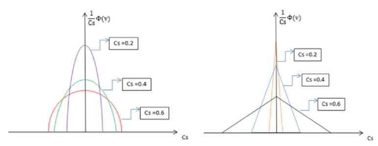
Fig. 1. Parabolic kernel

Fig. 2. Triangular kernel

Рис. 1. Параболическое ядро

Рис. 2. Треугольное ядро

At reconstruction of mutually ambiguous function of regression Nadaraya-Watson’s estimation has to be changed as follows [7; 8]:

Y s ( x t ) =

s

E у, ф

i = 1

xt - c

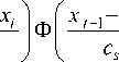
Ф f y t - 1 - y i - 1 I

I c s J

X i - 1 1 Ф f y t - 1 ^- y i - 1 1

J V c s J

x. — x,     f x, j -

> ф| -t----i- I ф I —t-1— i=1 V cs J V cs

, (9)

where x_{t– 1}, y_{t– 1} values of coordinates of regression function on the previous step of its estimation.

As numerous computing experiments showed it is worthwhile (7) to correct a bit as follows:

Y s ( X t ) =

s

E уф i =1

^xt ^-

xi

Ф0

f y t - 1 ^- y i - 1

V cs .

^Xi - 1 1 Ф о f y t - 1 ^- y i - 1 1

J V c s J

, (10)

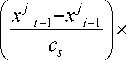
where Ф⁰( v ) with an accuracy to coefficient repeats Ф( v ), and Ф⁰( v ) = 1, if v < 1 and 0 in other cases. In this case Ф⁰( v ) will not affect a reconstruction error but will allow “to record” an algorithm in the previous point of the movement at estimation of every subsequent point. If x vector of dimension of k : ( x 1 , ^, x k ) e R k , the training sample in this case is: x_1i , ..., x_ki , y_i , i = 1, s. At reconstruction of mutually ambiguous function of regression nonparametric estimation has to be changed as follows:

^xt ^{- x}i

c

j x t -1

Y ⁽ x t ) = s _k

E№

J j = i V

^xt ^{- x}i

c

^f j -1-

C J

j

J j = 1 V

^Cs J

| y t - 1 ^- y i - 1

V cs   j yt -1 - y-11,(11)

cs    J where xjt–1, yjt–1 values of coordinates of regression function on the previous step of its estimation.

Nonparametric estimation (11) can be modified as follows:

s

E i = 1

kj

Уi П Ф⁰ | ^X2-

_xj _i

c

k

| П Ф 0

¹ j = 1

X ф 0 I ^yt - 1 ^- y i - 1

Y s ( x t ) =

cs

, (12)

s E i = 1

kj

П Ф^O | ^X^

-

c

jk x- Пф0

Х Ф 0 I y t - 1 ^- y i - 1

cs where Ф0(v) is same as above.

A computing experiment. First, we will consider some ideas of the control theory. The key feature is that the existing theory of control needs to present the object equation with an accuracy to a vector [9–11]. Proceeding from it, regulators can be synthesized: adaptive, selfadjusting and others [12; 13]. At application of the optimum theory of control [2; 14; 15] getting the regulators corresponding the given control task is possible. Blocks with the basic purpose of reconstruction of mutually ambiguous characteristics according to the experimental data can occur to be a constituent of the received control systems. We give the results of some computing experiment for a similar element of system below, exactly, the reconstruction of mutually ambiguous characteristics from observations. When carrying out a computing experiment mutually ambiguous characteristics can have various shapes: circles, ellipses and others. Without violation of generality, we will accept mutually ambiguous characteristic of dependence y(x) (for simplicity reasons) in the shape of a circle:

x 2 + y ² = r 2 ,                    (13)

where r – a circle radius.

In this case the training sample was formed in the following way: the initial point x' was set on a random basis and y'(x) was calculated according to (13). As a result, the sample x,, y,, i = 1, s was formed. Note that x, could be defined as a result of a stable step Ax on x e Q(x) or of a random number detector x e Q(x), i = 1, s . During the process of computer research other mutually ambiguous characteristics of dependence y(x) were also used.

At reconstruction of mutually ambiguous characteristic from observations unknown to the researcher, the question of the choice of the direction of movement is important, though, in principle, it can be arbitrary at an initial stage. But all subsequent changes of the current variable x are in rigorous dependence of the previous one.

The processes characterized by mutually ambiguous dependences have such feature that values x t , t = 1,2… appear strictly sequentially in this or that direction. In fig. 3 such process is presented. Let, for example, on the first step of x = x 1 , then x 2 etc. Values x t appear only after x t –1, that is “movement” x t in the arbitrary direction takes place. Emergence of values begins at some point of x_t and moves sequentially, passing points t ₂, t ₃ . At the same time transition of x ₁, for example, to x ₅ is impossible until the previous four points are passed. Thus, the entity of the offered estimates (9), (10), is that at estimation of the next point, “fixing” to the previous point in the corresponding algorithms takes place (9), (10).

In fig. 3 the process representing a circle is given. The movement along a variable happens from right to left and from left to right, what characterizes serial emergence of sample values.

On the following step random impact of h from observations yi was added h = lyfc,                      (14)

where ^ e [ - 1,1 ] , disturbances level l = 0,5,10 %.

As a criterion of accuracy of nonparametric estimation the ratio was used:

s

El y ^- y s ^{( x} i )l

w = ^---—,        (15)

E| y- y| i=1

1s where y = -У yt - arithmetic mean; ys(xi) - nonparas .=1

metric estimation; y_i – true sample received according to a formula (13).

We will give the results of a numerical research illustrating effectiveness of an algorithm. As a bell-shaped finite function the triangular kernel was used. The algorithm was tested on the training samples of various sizes, at the same time serial increase in a sample size was performed by addition of new elements to already available: s = 50, 100, 500.

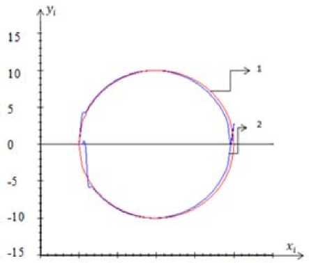
In all drawings we designate figure (1) – the training sample, (2) – nonparametric estimation.

The operation of an algorithm (9) in fig. 4–6 under various conditions is shown: when the sample size is equal to 50, 100, 500 elements; the disturbances level is equal to 0 %; the experiment was conducted in the mode of the sliding examination.

In fig. 7 the dependence of an error values of reconstruction of size at various disterbance levels is presented.

In computing experiments other mutually ambiguous characteristics were also used. Some fragments of a research are given below. In fig. 8, 9 the experiment under various conditions was conducted: the sample size is equal to 100, 200 elements; the disturbance level is equal to 0 %; the experiment was made in the mode of the sliding examination.

In fig. 10–15 it is well visible how the error of reconstruction depends on a disturbance level and on a sample size for a circle and for amore composite figure.

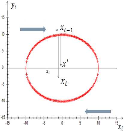
Fig. 3. This sample is presented

Рис. 3. Представлена данная выборка

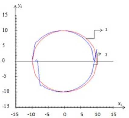
Fig. 4. S = 50; w = 0.1098

IS -10 -S 0 S 10    15

Fig. 5. S = 100; w = 0.0469

Рис. 4. S = 50; w = 0,1098

Рис. 5. S = 100; w = 0,0469

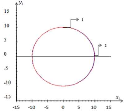
Fig. 6. S = 500; w = 0.0068

Рис. 6. S = 500; w = 0,0068

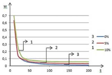
Fig. 7. Dependence of the recovery errors on the volume at different levels of interference

Рис. 7. Зависимость значений ошибки восстановления от объема при различных уровнях помех

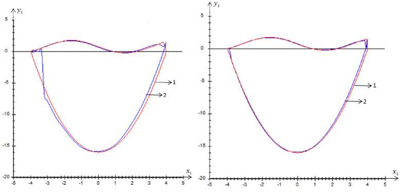
Fig. 9. S = 200; w = 0.018

Fig. 8. S = 100; w = 0.042

Рис. 8. S = 100; w = 0,042

Рис. 9. S = 200; w = 0,018

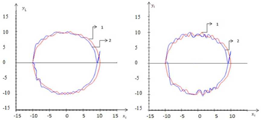
Fig. 10. S = 50; l = 5 %; w = 0.2173                   Fig. 11. S = 50; l = 10 %; w = 0.2926

Рис. 10. S = 50; l = 5 %; w = 0,2173                  Рис. 11. S = 50; l = 10 %; w = 0,2926

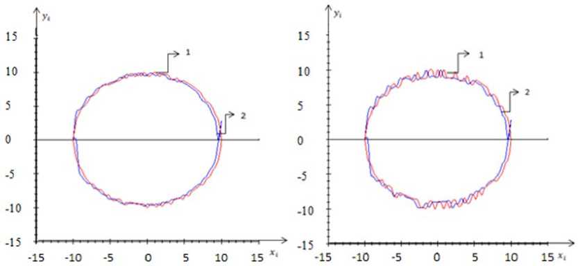
Fig. 12. S = 100; l = 5 %; w = 0.0602        Fig. 13. S = 100; l = 10 %; w = 0.0845

Рис. 12. S = 100; l = 5 %; w = 0,0602        Рис. 13. S = 100; l = 10 %; w = 0,0845

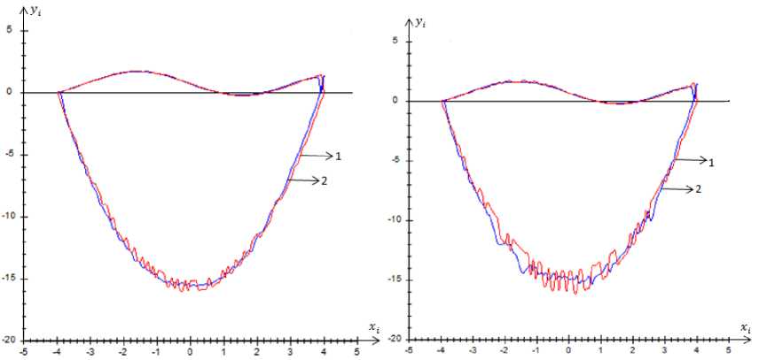
Fig. 15. S = 200; l = 10 %; w = 0.0011

Fig. 14. S = 200; l = 5 %; w = 0.0308

Рис. 14. S = 200; l = 5 %; w = 0,0308

Рис. 15. S = 200; l = 10 %; w = 0,0011

For descriptive reasons, we will change places of y i and x i in estimation (9) in fig. 16, 17. We will be convinced that estimation differs a bit at points of intersection of the graph and an abscissa axis as could seem from fig. 10–13.

We will demonstrate the work modified algorithm (10), under the following conditions: at a disturbance level equal to 5 and 10 %; with a sample size equal to 100 elements; in the mode of the sliding examination. Comparing errors of reconstruction we look at fig. 12, 13 and 18, 19 and we see a small improvement.

In fig. 18, 19 we see that an error of reconstruction is a little less than in fig. 12, 13. This means that nonparametric estimation has became more accurate.

Also in a case with a more composite function in fig. 20, 21 it is visible that an error of reconstruction is a little less than in fig. 14, 15. This means that nonparametric estimation has became more accurate.

It should be noted that: with decrease of an error reconstruction ( w ) the accuracy of estimation increases; with the increase of a sample size ( s ) the error of reconstruction ( w ) decreases; the size of an error grows at increase of a disturbance level (l).

The following question is possible: “Why was the circle used to check the work of an algorithm?”, because there are a lot of more composite shapes, and the answer is simple – the chsracteristic of this algorithm is its universality. This means that it is not essential for an algorithm what function to reconstruct, whether it is a circle, an ellipse, an Archimedes spiral or a Cassini’s oval. “Being fixed” in the previous x t point, that is in a x t– 1 point, and following the sense of a rotation, it is always possible to get a nonparametric estimation of mutually ambiguous functions.

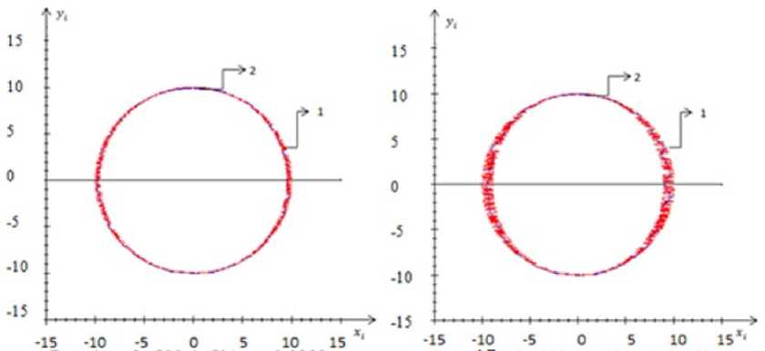
Fig. 16. S = 500; l = 5 %; w = 0.0283

Рис. 16. S = 500; l = 5 %; w = 0,0283

Fig. 17. S = 500; l = 10 %; w = 0.055

Рис. 17. S = 500; l = 10 %; w = 0,055

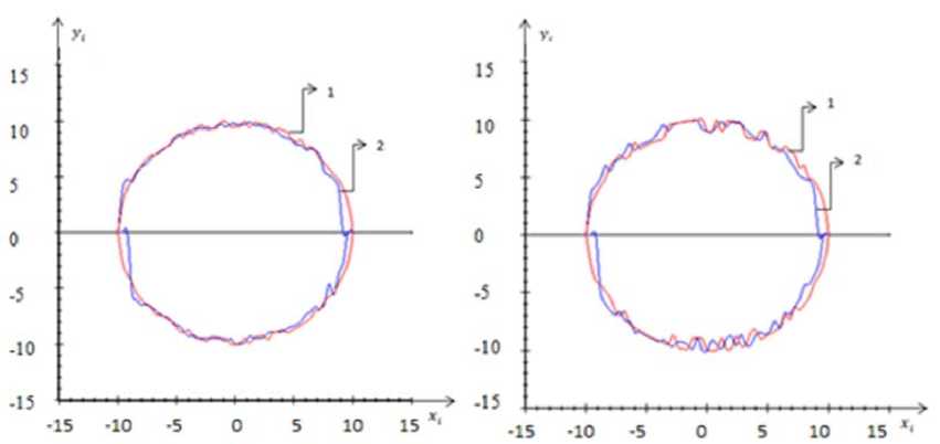
Fig. 18. S = 100; l = 5 %; w = 0.057

Рис. 18. S = 100; l = 5 %; w = 0,057

Fig. 19. S = 100; l = 10 %; w = 0.0817

Рис. 19. S = 100; l = 10 %; w = 0,0817

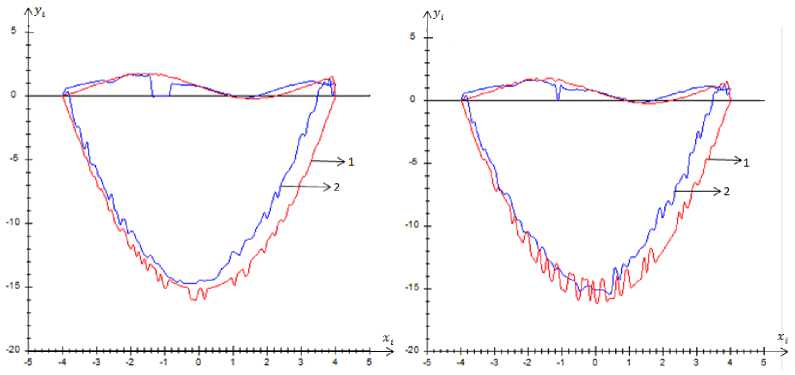
Fig. 20. S = 200; l = 5 %; w = 0.0301

Рис. 20. S = 200; l = 5 %; w = 0,0301

Fig. 21. S = 200; l = 10 %; w = 0.0009

Рис. 21. S = 200; l = 10 %; w = 0,0009

Conclusion. The main result of the present article is an introduction of a new class nonparametric estimation of mutually ambiguous functions from observations with errors. It distinguishes the problems of nonparametric estimation from the known nonparametric estimates of the function of Nadaraya-Vatsona regression . Some modifications of nonparametric estimates are given, under such conditions the attention is drawn to a method of bypassing of entered nonparametric estimates along a trajectory determined by elements of the training sample.

For simplicity of a numerical research the function described by a circle was taken, though it is not essential to the offered algorithm. In other words, the algorithms offered are suitable for reconstruction of the ambiguous dependences described by more composite curves, the character of which is apriori unknown, only a sample of observations of the studied process is known.