Nonlinear Gust Response Analysis of Free Flexible Aircraft

Published Online January 2013 in MECS

Modern aircraft design requires the evaluation of dynamic loads in response to discrete and random gust excitations. Gust response affects many aspects of aircraft characteristics, including stability and control, dynamic structural loads, flight safety and easement. The Federal Aviation Regulations require that the aircraft structure can withstand discrete gusts of certain profile, intensity and gradient [1]. Because of its multidisciplinary nature with aerodynamics, flight mechanics, aeroelasitcity, and atmospheric turbulence, until now, only the doublet-lattice, unsteady linear aerodynamic cod DLM, coupled with the equation of motion of flexible vehicle, was used for gust response analysis [2-5].

Flight mechanics and aeroelasticity can be often treated as separate discipline, namely, flight mechanics and aeroelasticity. The first one concerned principally with rigid aircraft experiencing large motions (commonly known as Rigid Body Approximation-

RBA), while the second aims mainly to the analysis of elastic aircraft experiencing relatively small deformations. The idea to not consider cross-coupling effects between these two disciplines has been commonly justified by the large frequency separation of the characteristic motion which is typical of conventional structures. Nowadays, the focus on weight minimization for aircraft, leads toward more and more flexible vehicles. The resulting underlying structures may not exhibit the usual wide frequency separation among the rigid body degrees of freedom and the remaining elastic modes. So that the approach mentioned above can lead to mistakes/errors in analyses of flight performance, flying qualities, and control systems design. In these cases, an integrated analysis of flight mechanics and aeroelasticity is necessary from the very early stages of preliminary design [6].

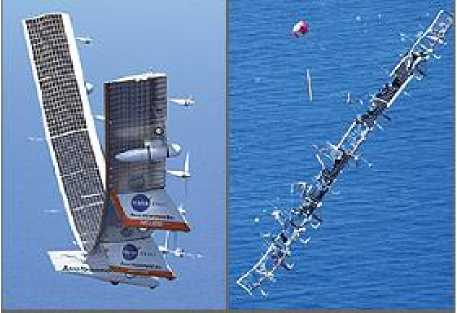
Fig. 1: HP03-2 mishap

Another reason which substantiates the development of an integrated approach is high-altitude; long-endurance (HALE) unmanned aerial vehicles (UAVs) are recently receiving considerable attention from the technical community. Patil [7], Shear [8], Cesnik and Weihua Su [9-10] showed that when the nonlinear flexibility effects are taken into account in the calculation of trim and flight dynamics characteristics, the predicted aeroelasitc behavior of the complete aircraft turns out to be very different from what it would be without such effects. The Helios accident also highlighted our limited understanding and limited analytical tools necessary for designing very flexible aircraft and to potentially exploit aircraft flexibility. The number one root cause/recommendation from NASA

[11] was “more advanced, multidisciplinary (structures, aeroelastic, aerodynamics, atmospheric, materials, propulsion, controls, etc.) time-domain analysis methods appropriate to highly flexible, morphing vehicles [be developed].”

For all of the reasons stated, a better understanding of the flight dynamics/aeroelasticity of these vehicles is required. The key points are the aerodynamic loads as well as the mass distribution. During flight the maneuvers change the aerodynamic loads which act on the aircraft. Thus a variation on the structural displacements is expected, modifying the mass distribution and therefore the inertia moments, important parameters for the characterization of the aircraft dynamics. The structural displacements cause also a variation on the aerodynamic loads through the alteration of the body geometry and due to motion (its time derivative). Although there are commercial software tools capable of dealing with pieces of the problem, there is no commercially available software that integrates all of the disciplines needed for such investigation as discussed here.

The intention here is not to investigate complex flight mechanics behavior, but to describe the development of a tool which can be used for this purpose. This paper illustrates a multidisciplinary coupled numerical tool to simulate detailed aircraft models undergoing arbitrary free flight motion in the time domain, by Computational Fluid Dynamics (CFD), Computational Structure Dynamics (CSD) and Computational Flight Mechanics (CFM) coupling. A substantial part of this work is devoted to the development of an integrated aircraft flight mechanics model as generic as possible, which comprises the structure vibration influence, without loss of : the simplicity of the equations; the similarity to the classical RBA; and perhaps the most important, the physical understanding of the interactions. The modal decomposition technique is used to represent the structural dynamic [12]. The CFD solver developed by MFDCL (Multidisciplinary Flight Dynamic and Control Laboratory, College of Astronautics, Northwestern Polytechnical University), will be used to compute the unsteady aerodynamics loads in this work.

II. Numerical Approach

2.1 Flight Model

A finite element analysis using Patran/Nastran is assumed to have been performed, such that a modal description of the structure is available. That is, if the

elastic deformation at position(x, y, z) on the structure is denoted as d , then it may be written as

го d=Хф( x, y, z )П i=1                                                      (1)

n.

where is a generalized coordinate of the structure

and ^{ф (} x , y ■ z )

is a mode shape. Of course, a finite

number of modes must be used, so that the model

always is based on a truncated-mode description.

The equations of motion are developed with the use of a special body-reference axis, the axis referred to by Milne as the mean axis. This axis is the coordinate frame with respect to which the elastic deformations contribute no translation or rotation momentum. For the mean axis, the following relations hold:

I л pdV=!p x л pdV = 0

where an infinitesimal volume of the vehicle d V has location p with respect to the instantaneous center of mass of the vehicle. All of the equations of motion are derived using this body-referenced (mean) axis, and all forces, moments, and inertias must be resolved into components along and about the three directions, that is, x, y, and z of this axis.

The dynamic equations of motion for the elastic aircraft are then derived from first principles using Lagrange’s equation [13]:

+— = Qi ^d q   d q_t

The resulting equations from the application of Eq. (3) may be expressed as follows:

Equations for rigid-body translational accelerations:

M ( U + qw - rv + g sin 0) = X

Equations for rigid-body rotational accelerations:

Ixp - (Ixyq + Ixzr) + (Iz - Iy )qr + (Ixyr - Ixzq)P + (r2 - q2 )Iyz = L Iyq - (Ixyp + Iyzr) + (Ix - Iz )Pr + (IyzP - Ixyr)q + (P2 - r2 )Ixz = M Izr - (Ixzp + Iyzq) + (Iy - Ix )pq + (Ixzq - IyzP)r + (q2 - P2)Ixy = N

Equations for elastic degrees of freedom:

п + 2 ?м + to^ i = q mm^i

• 2.2    CFD Solver

• 2.3    Coupled Solution Procedure

The behavior of the fluid flow affecting the object of interest is simulated with the EU3D-Code, a CFD tool developed by the Multidisciplinary Flight Dynamics and Control Laboratory. A full discussion of the code and turbulence models implemented is given in reference [14]. The EU3D-Code solves the compressible, three-dimensional, time-accurate Euler and RANS equations using a finite volume formulation. The Code is based on a structured-grid approach. The grids used for simulations in this paper were created with the grid generator Gridgen. The Code contains several upwind schemes, FDS-Roe, FVS-Vanleer, AUSM+ and AUSMpw+. LUSGS and dual time step marching scheme LUSGS-T TS is also available.

The coupling flow chat is showed in Fig.2:

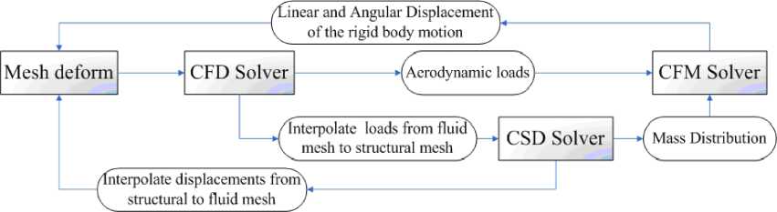
Fig. 2: CFD-based multidisciplinary coupled numerical simulation flow chart

The detail coupling algorithm is:

• (a)    The CFD solver computes a set of aerodynamic loads based on the mesh at a new time step;

• (b)    Interpolate aerodynamic loads from fluid mesh to structural mesh;

• (c)    The CSD solver uses the interpolated loads to compute the structure responses for the current time step, according to Equation (6);

• (d)    Compute the center of mass and the inertia tensor based on the mass distribution;

• (e)    The CFM solver uses the aerodynamic loads from the CFD solver and the mass characteristic to compute the flight dynamic response, according to Equation (4) and (5);

• (f)    Update the fluid mesh based on the structure and flight dynamic response, and send the updated mesh to the CFD solver;

• (g)    The loop goes back to point (a), until the desired condition is reached.

In the current implementation, the CFD solver takes care of computing the resultant forces and moments, and the generalized forces from the pressure distribution. When the CFD solver converges, it stops sending aerodynamic loads information and waiting for the updated fluid mesh information. The equations of flight dynamics and structure dynamics are solver by four-order Runge-Kutta method.

CFD-CSD Interface. Generally, the CFD-CSD interface refers to the transformation to the structural grid of aerodynamic forces that are computed on the aerodynamic grid, and to the mapping of the elastic deformations computed on the structural finite element nodes to the aerodynamic grid. When the modal structural approach is taken, with the structure represented by a set of its low-frequency vibration nodes, the CFD-CSD interfacing task reduces to mapping the modes to the aerodynamic surface grid points. After this is done, the computation of elastic deformations can be carried on within the fluid dynamics computations. The Infinite Plate Spline (IPS) method by Harder and Desmarais is applied to exchange the boundary information between the fluid mesh and the structure mesh [15]. Fig.3 shows 30 times mode shapes mapped into CFD surface grid.

Mode1                     Mode2

Mode3                     Mode4

Fig.3: First four elastic mode shapes mapped into CFD surface grid

Aerodynamic Grid Update . The gird must be deformed once per time step in unsteady flow simulations. Once the aerodynamic surface grid points have been deflected to account for the control surface deflections and the rigid motion of the aircraft, the grids must also be deflected accordingly. A modified TFI method is employed here. The main ideas about the TFI method of grid perturbations are described in reference [14].

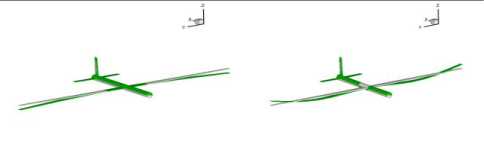
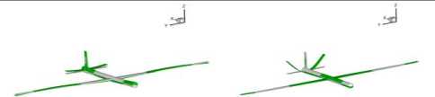
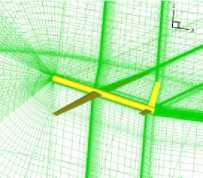
It should be noted that the longitudinal 3DOF equations are loosely coupled, in that they are solved sequentially for each time step. With the new CG locations and pitch attitude, the grid is rigidly translated and rotated accordingly, and the grid velocities are computed using second order finite differences. The process is illustrated in Fig.4 for a generic aircraft test case with an all moving elevator. Fig.5 shows that after the rotation of the aircraft, the flow girds were updated by TFI.

reaction appears. The aircraft is considered as trimmed when vertical reaction force and pitching moment are null. A deflection of the elevator is then used to guarantee the final equilibrium of vertical force and pitch moment. Fig.6 shows the CFD mesh used for Euler calculations. The complete aircraft is modeled, despite symmetric flow conditions are considered in the following examples. An all-movable elevator is introduced in this case; the detail grid is outlined.

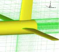
a) Original Surface Grid

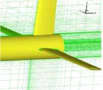
b) Elevator Deflected

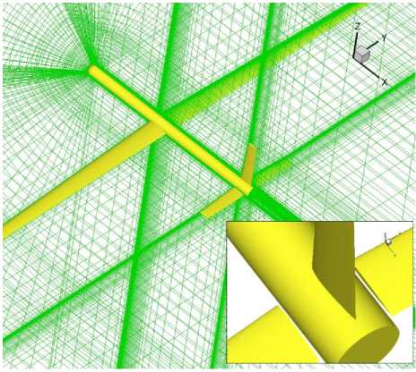
Fig. 6: The CFD mesh and elevator detail used for the numerical simulation

Fig.4: Deflection of the elevator

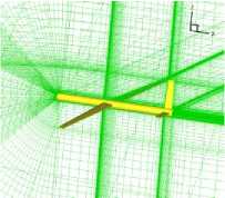
a) Original grid

b) Rotated Grid (TFI)

Fig.5: Rotation of the aircraft

The solution of the trim problem is iteratively sought in a manner as outlined in Fig.7; it consists of three different nested iteration-levers [12]:

The Basic Level. Considering the aircraft is rigid, a maneuver trim loop adjusts elevator deflection and aircraft attitude to have the static equilibrium position is sought. In this case, M iterative loop is introduced to solve the Eq. (7) for symmetric maneuver.

2.4 Trim Process

So far we have obtained a multidisciplinary coupled numerical tool to simulate the flexible aircraft in timedomain. The next step is generally necessary to first solve the so-called trim problem. For rigid body approximation, the trim problem can be characterized in the following way: find a set of suitable input values, e.g. aircraft angle of attack, elevator setting, thrust, to satisfy a set of conditions, e.g. to fly in a straight path in steady state, i.e. no accelerations along x , z , and no rotational acceleration around y . For the elastic aircraft, an additional condition to the conventional trim requirements is that the elastic deformation is in steady state, i.e. the second derivatives of all body motion representing the elastic structure have to be zero [16].

In this case, the effect of thrust on the trim configuration is neglected and a non-null horizontal

"s§

+

4 S

Z i s

M

4 §

Me

F z,res

У, res

FM

Where ^{z , res} and ^{y , res} refer to the

residual of non-

dimensional flexible normal force and pitching moment terms that correspond to a current set of values of trim

parameters. The value of

C S , C § ( i = L , M )

may be

known experimentally or through the CFD solver. Including aeroelastic effects on these derivatives using the CFD solver leads to further computational costs. Thus for this simple application, their values are never updated and determined once for all starting from the undeformed reference condition of null pitch and elevator deflection. Of course, this leads to a slower

convergence for trim corrections.

The Medium Level. Once the ^M iterations reached, assuming the variables giving the motion of the aircraft and its controls in the body reference frame as frozen, the deformed trim shape for the current configuration is sought. A user-defined number of iterations N is carried out:

Kn ^{( / + 1)} =Q ( n ⁽⁰, x ⁽ n ) , 8 ^{( n} ) )

After N iterations, the solution may not be the final equilibrium point between elastic and aerodynamic forces dependent on the assumed structural configuration, but it doesn’t matter.

The Outer-most Level. This level simply is executed until overall convergence is reached.

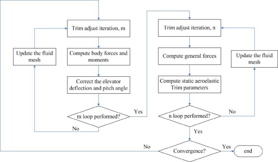
Fig.7: flow chart for the deformable trim process

• 2.5 Field Velocity Method and Validations

The so-called field velocity approach, developed by Baeder[17,18], is used to calculate the gust response. The field velocity approach can be considered as an extension of the surface transpiration approach. The velocity correction is applied throughout the flow field as opposed to only on the surface as in the surface transpiration method. Mathematically, the field velocity approach can be explained by considering the velocity field ^V in the computational domain. It can be written as:

V = ⁽ u - x T ) i + ⁽ v - y _T ) j + ⁽ w - z T ^{) k}      (9)

Whereu, vandware the components of the velocity along the coordinates directions and T, yT, and ^T are the grid time metric components. For the flow over a stationary wing these components are zero. Let a gust

w be represented by velocity g along the z direction

(Fig.8). Thus, the velocity field becomes:

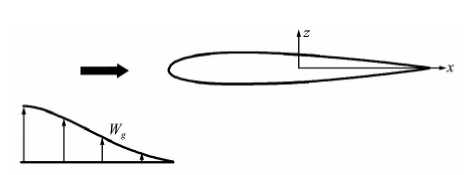
Fig. 8: Sketch of gust response on a wing

This simply velocity correction approach, besides being free of numerical oscillations, provides a way to directly calculate the indicial responses of an airfoil with respect to step changes in angle of attack and pitch rate, as well as the penetration of a sharp-edged gust, but the mesh is not moved accordingly.

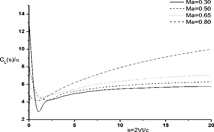
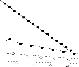
Specific computations were performed for a NACA0006 airfoil at free stream Mach numbers ofMда 0.3,0.5,0.65 and o.8 with a gust velocity equal to 0.08 times the free stream velocity, such that it induced a net change in angle of attack of approximately 4.57 degree in each case.

V =(u - XT )i+ (v - Ут)j+ (w - zT + wg)k (10)

(a) Lift coefficients

C/ α 8

Exact,M=0.3

• ■  CFD, M=0.3

Exact,M=0.5

• •  CFD, M=0.5

Exact,M=0.65

о  CFD, M=0.65

Exact,M=0.8

CFD, M=0.8

2 J—I-0.0

0.2

0.4           0.6

s=2Vt/c

0.8

• (b) Comparison with exact results

Fig. 9: Results of the sharp-edge gust response using CFD

Fig.9(a) shows the computed coefficients of lift for the sharp-edge gust response, as a function of the non- s = 2V / c dimensional aerodynamic time     ∞

.

Fig.9(b) shows a comparison of the computed and exact results at small times. It can be seen that the agreement is excellent. The unsteady flow computation and gust response analysis by CFD adopted here are validated by these computations.

• III.    Numerical Model and Results

  • 3.1    Aircraft Model

Because it is hard to find the structural data of a flexible vehicle, a wing-body-tail aircraft configuration with slender wings (aspect ratio 33.33) designed by the author, as shown in Fig.10, which may not be reasonable, is selected as a test case for the numerical simulation. The total length of the fuselage is 30m. The detail geometric properties and mass properties are included in Table 1 and Table 2, respectively.

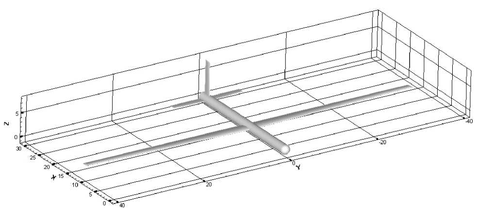
Fig. 10: Slender-wing HALE aircraft configuration

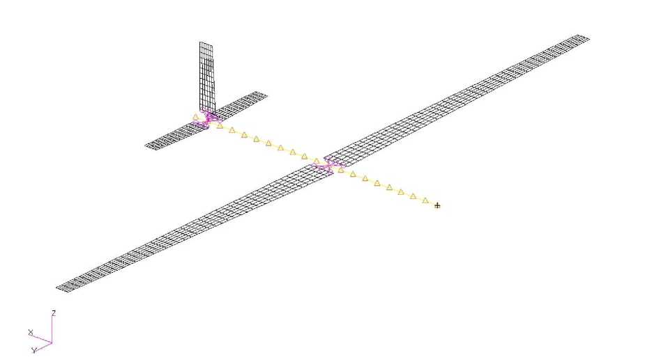
Fig. 11: Structural model of the aircraft

Table 1: Geometry of The Slender-Wing Model

	Wing	HTP	VTP
Span	75m	16m	8m
Root Chord	3.0m	2.0m	2.0m
Tip Chord	1.5m	1.2m	1.2m
Airfoil	NACA 4415	NACA 0012	NACA 0012
Incidence Angle	2.0°	2.0°	0°
Wing Area: 168.75m2                                   Wing-to-HTTP: 15m Wing-to-Nose: 12m

Table 2: Inetia Properities

Center of mass	x = 13.808743 m , y = 0.0 m , z = 0.021649 m c    cc
Pitching moment of inertia	Iyy = 8.17175 × 105 kg ⋅ m 2
Total mass	12091.605469kg

In the modeling of the FEM, the fuselage is modeled as a beam. The wing, the elevators and the vertical rudder are modeled as shell element, and contacted with the fuselage by MPC, the FE model is presented in Fig.11.

As an example for the coupled simulation, a one-minus-cosine gust has been defined. In detail, to reduce the complexity of the problem, a symmetric flight condition has been considered. The reference flight condition is Mach 0.5 at sea level. The simulation has been performed both with a rigid and with an elastic model. One goal of the simulations is to assess of the differences between the two approaches, most notably to see whether an elastic model has an influence on the prediction of the aerodynamic loads and the flight properties.

An incrementally complex problem has been considered:

• a)    The aircraft is first trimmed in a desired flight condition, by computing the pitch ,elevator settings and the structure deformation for level flight;

• b)    A one-minus-cosine gust starting from the trimmed flight condition is considered, with the aircraft constrained by a revolute joint about the pitch axis.

• c)    The same gust velocity profile is considered, with the aircraft constrained only by symmetry constraints (vertical and longitudinal displacement, pitch rotation); Thrust is assumed to be an applied force on the aircraft center of gravity that compensates the horizontal forces on the trimmed condition.

• 3.2    Trim Results

0.06 0.04 0.02 0.00

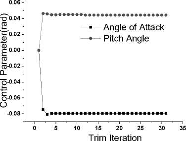
In case of a stationary, straight symmetrical flight, all asymmetric equations of motion reduce to zero. Two cases were considered, the rigid-run and elastic-run. In this work, the iteration number ^{M = N = 5} , the ending

.

conditions is .For the rigid-run, Fig.12 shows the convergence history of the trim problem for the rigid run.

-0.02

-0.04

-0.06

-0.08

--■-- angle of attack

—•— pitch angle

0   2   4   6   8   10  12  14  16  18  20

Τ rim Iteration

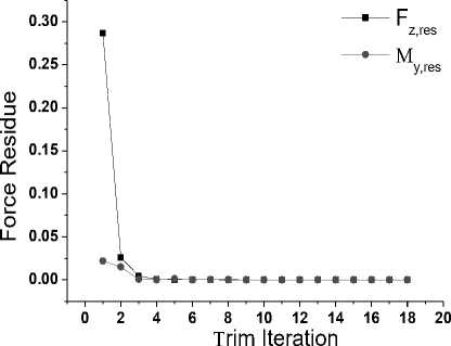
(b) Residual of the normal force and moment coefficient

(a) Trim variables at each iteration

Fig. 12: Convergence of the trim problem for the rigid-run

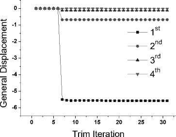
Fig.13 presents the convergence of the trim problem of the elastic-run. Fig.13 (a) briefly reports the pitch angle ψ and elevator deflection ^e at trim iterations, Fig.13 (b) shows the value of modal displacements at each iteration for the elastic solution. Table 3

summarizes the trim states of the rigid-run and elasticrun, which indicates that the trim states are nearly unchangeable with or without the consideration of the structural deformation due to the stronger structural mass and rigidity of the aircraft.

(a) Trim variables at each iteration

(b) Values at each trim step iteration

Fig. 13: Convergence of the trim problem for the elastic-run

Table 3: Trim States Comparsion

	ψ/ rad	δ e /rad
Rigid-run	-0.079497	0.045009
Elastic-run	-0.079528	0.0443999

Table 4: Trim States Comparsion

	General displacement
	1st	2nd	rd	4th
Rigid	0	0	0	0
Elastic	-5.58316	-0.680013	-0.120040	-0.0151869

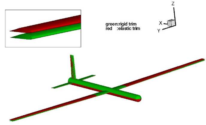
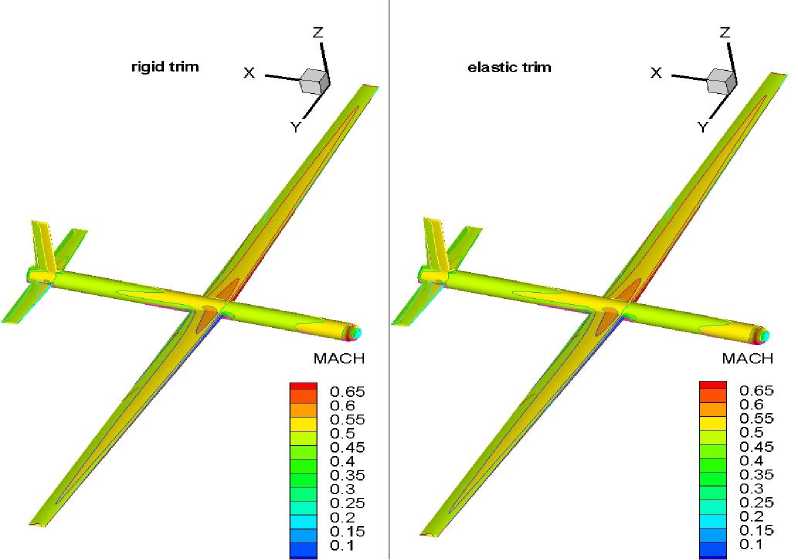
The final deformed shape is depicted in Fig.14 (a).

Fig.14 (b) shows the difference in chord-wise Mach distribution for the rigid and deformable trim configurations.

(a) Final deformed shape

(b) Mach distribution at trim state

Fig. 14: Comparison of trimmed state between the rigid-run and elastic-run

• 3.3    Free-to-pitch Simulation

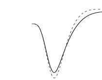
In general, gust disturbance is stochastic. In this paper, the gust model is simplified as a discrete gust having one-minus-cosine velocity profile, namely, wg = — w0 [1 - cos (2ntJ2T)]

²                                     (11)

w

• ⁰ is the design cruise gust velocity. Before and after the discrete gust pulse, there is no gust flow perturbation. The velocity profile is shown in Fig.15.

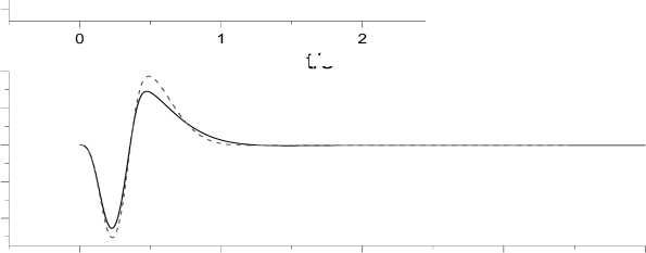
The response of the pitch angle and its’ rate are shown in Fig.16 for a rigid and elastic aircraft. The initial pitch is completely recovered after the pulse response is removed. This analysis shows that the ‘short-period’ (pitch) motion of the aircraft is stable. The time histories of load coefficients of lift, drag, pitching moment are shown is Fig.17. Fig.18 shows

C the m history as a function of angle of attack, which indicates that although the rigid-run and the elastic-run both recovered to the equilibrium state, the time history and hysteresis effect are still different.

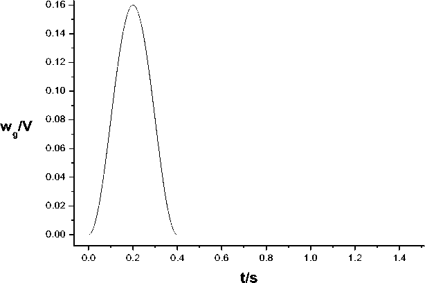
Fig. 15: Time variation of gust speed

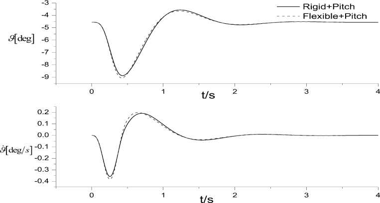
Fig. 16: Pitch rotation and rate

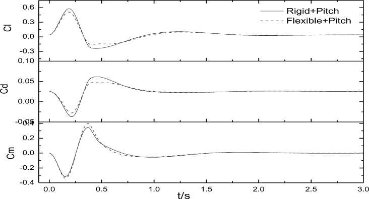
Fig. 17: Time histories of the coefficients of lift, drag and pitching moment

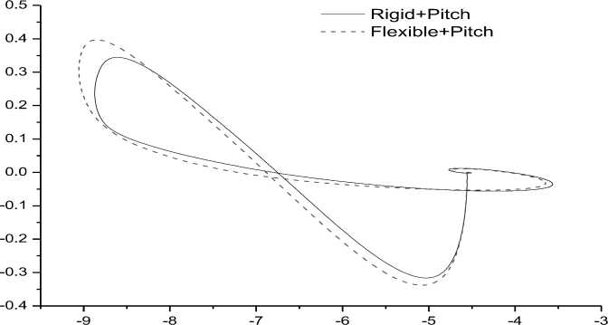
Fig. 18: Pitching moment history as a function of angle of attack

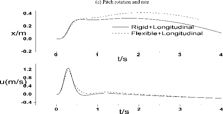
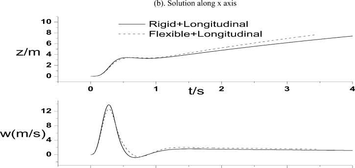
• 3.4    Free-Flying of the Longitudinal Flight

With the same gust velocity profile, the displacement in translations, plunging and the angular displacement in pitch are shown in Fig.19. As illustrated by these figures, the free model ends up in an almost steady ascent. The motion of the aircraft should evolve into a ‘phugoid’ transient (altitude/horizontal speed oscillation). However, the duration of the period is much longer than what one would expect to capture with this type of analysis.

^ [ deg ] "5

-6

Rigid+Longitudinal

Flexible+Longitudinal

-7

0.2

0.1

0.0

^ [ deg/ ^ ]

-0.1

-0.2

t/s

2 t/s

t/s ²

(c). Solution along z axis

Fig.19: Response for the free flying case

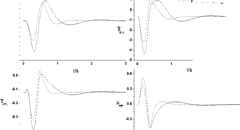
Fig.20 shows the time histories of the coefficients lift, drag and pitching moment. Fig.21 gives the time histories of structural deformation of the generalized displacements. The structure deformation occurs mainly in the first two modes, which corresponds to the first and second bending modes of the wing. After the pulse response, structural deformation oscillates to revert to the original equilibrium state for the free to pitch, when take into account of the plunging and translation, the structure deformation oscillates to a new equilibrium state faster. Fig.22 shows the time history of pitching moment of inertia, it varies with the structure deformation, and indicates that the mass distribution of the aircraft.

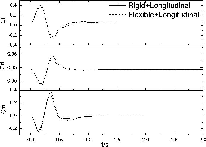
Fig. 20: Time histories of the coefficients of lift, drag and pitching moment

-20

-40

-60

-80

Flexible+Pitch

Flexible+Longitudinal

-0.4

-0.6

t/s t/s

• Fig. 21:    Time histories of structural deformation of the first four symmetric modes for the flexible configuration

  
  

  Rigid
  
  Flexible+Pitch
  Flexible+Longitudinal

  
  
  
  
  
  

  CN “  820000

  E □)           ■

  
  
  

  0.0         0.4         0.8

  
  

  -1-------¹-------Г"

  1.2          1.6

  
  

  -1-------¹-------Г"

  2.0         2.4

  
  

t/s

• Fig. 22:    Time history of the pitching moment of inertia for the aircraft

• IV. Conclusion

In the present paper, a multidisciplinary coupled numerical tool to simulate detailed aircraft models undergoing arbitrary free flight motion in the time domain was illustrated. The simulation tool combines time-accurate aerodynamic, aeroelastic and flightmechanic calculations to achieve this objective. This type of problems requires the use of sophisticate fluiddynamics models, in order to capture the relevant dynamic effects of unsteady transonic flow, including aerodynamic loads that depend on unsteady compressibility effects.

The numerical tool uses an advanced coupled computational fluid dynamics (CFD), computational structural dynamics (CSD), and computational flight mechanics (CFM) technique that provides for a gird motion capability to fly an elastic aircraft on the supercomputers.

A novel method for CFD-based maneuver trim analysis was presented. The method belongs to the category of closed coupled aeroelastic analyses, in which the flow analysis, elastic deformations, and trim computations are performed within the CFD code, within a single run. The results of trim and transient analysis applied to a slender wing HALE aircraft show the soundness of the proposed procedure.

Acknowledgments

The authors would like to thank the anonymous reviewers for their careful reading of this paper and for their helpful comments. This work was supported by the National Natural Science Foundation of China under grant no. 90816008 and Doctoral Fund of Ministry of Education of China under grant no.20070699054.