Numerical Implementation of Nonlinear Implicit Iterative Method for Solving Ill-posed Problems

Published Online August 2011 in MECS

This paper is dedicated to the computation of an approximation to a nonlinear operator equation

F(x) = y,                            (1)

where F:D(F) X ^ Y is a nonlinear operator between two real Hilbert spaces X and Y. If only noisy data y^δ with

II y5-y II < 5                                  (2)

are available, then the problem of solving (1) has to be regularized. Nonlinear ill-posed problems are more different to solve than linear. Due to the importance for technical applications, many of the known linear regularization methods have been generalized to nonlinear equations[1,2].

In [3], we extend the implicit iterative method for linear ill-posed operator equations to solve nonlinear ill-posed problems, named nonlinear implicit iterative

Footnotes: 8-point Times New Roman font;

Manuscript received January 1, 2008; revised June 1, 2008; accepted July 1, 2008.

Copyright credit, project number, corresponding author, etc.

method. Under some conditions, the error sequence of solutions of the nonlinear implicit iterative method is monotonically decreasing. And with this monotonicity, we prove the convergence of our method for both the exact and perturbed equations. In this paper, we focus on the numerical implementation of nonlinear implicit iterative method. The main part in the numerical implementation is how to minimize the Tikhonov functional in each iteration. When regularization parameter is fixed, how to minimize the Tikhonov functional (3) is a well-posed optimization problem. In principle, all of nonlinear optimization methods can be implied to implement the nonlinear implicit iterative method. But, the convergence may not be hold since the local convergence of some methods and the non-strictly convex of the Tikhonov functional.

J a (x)= II y ⁵ - F(x) II ² +a II x- x o II ²           (3)

In the numerical implementation of nonlinear implicit iterative method, we combine this method with the steepest descent method and develop an iterative algorithm for solving nonlinear ill-posed problems. It maintains the advantage of iteration methods in numerical realization and get a convergence result under some not very strict assumptions. In every iteration, we modify Tikhonov functional by idea of nonlinear implicit iterative method, replacing x⁺ with x^δ n :

J a (x, x⁵)= II y ⁵ - F(x) II ² + a II x- x II ²          (4)

The resulting method will be defined by x5,k+1 = x . + ek▽ Ja(x ., x )                   (5)

Here, βk denotes a scaling parameter. Since it is based on the interaction of nonlinear implicit iterative method with the gradient method, we feel that 'Implicit Iterative-GRAdient method ' (IIGRA) is an appropriate name for the iteration.

The structure of the paper will be as follows. In section II, it will be shown that the modified Tikhonov functional (4) has a convexity property in the neighbourhood of a global minimizer of the functional. A convergence analysis for the steepest descent algorithm for minimizing (4) is given in section III. It is shown that the algorithm converges to a global minimizer of (4) if a starting value for the iteration within the abovementioned neighbourhood is known. Finally, in section IV, we will give two applications. Conclusion is in section V.

• II.    Results On The Convexity Property Of Modified Tikhonov Functional

Throughout this paper we have the following assumption:

Assumption 1 Suppose there is a ball B(x⁺, r) ⊂ D(F) with radius r around x⁺ and in the ball operator F satisfies:

• (i)    F is twice Fréchet differentiable with a continuous second derivative;

• (ii)    local Lipschitz condition: for x₁, x₂ ∈ B(x⁺, r) there holds

‖ F'(x 1 )- F'(x 2 ) ‖ ≤ L ‖ x 1 -x 2 ‖ ;            (6)

• (iii)    ∃ some const η > 0, for all x 1 , x 2 ∈ B(x⁺, r) there holds

‖ F(x 1 )-F(x 2 )-F'(x 2 )(x 1 -x 2 ) ‖ ≤η ‖ x 1 -x 2 ‖‖ F(x 1 )-F(x 2 ) ‖ ;

As a deduction, we can conclude that F' is local bounded in B(x+, r) from assumption 1 (i), i.e.

M = sup{ ‖ F'(x)|x ∈ B(x⁺, r) ‖ } < ∞      (7)

Our aim is to use the steepest descent method for minimizing J α (x, x n ^δ ). It is well known that the steepest descent method will converge to (the global) minimizer of a functional, if it is convex. So we will prove that the modified Tikhonov functional has a convexity property in the neighbourhood of a global minimizer of the functional. Since limited by pages, we only give the convergence results without proof in the following, detail seen in [4].

From now on we will set

C x (t)(h, h):=∫¹ 0 (1-τ) F''(x + tτh)(h, h)dτ.       (8)

By Taylor formula in integral form

F(x + th)=F(x) + tF'(x)h+∫¹ 0 (1-τ) F''(x + tτh)(h, h)dτ, we have

F(x+th)=F(x)+tF'(x)h+t²C x (t)(h,h).        (9)

Let

φ α,h (t)= J α (x n ^δ +1 +th, x n ^δ ),t ∈ R, h ∈ X, ‖ h ‖ =1 , using (9) we get

J α (x+th, x n ^δ )=J α (x, x n ^δ )-2t( 〈 y^δ-F(x),F'(x)h 〉 -α 〈 x-x n ^δ , 〉 ) +t²( ‖ F'(x)h ‖ ²-2 〈 y^δ-F(x), C x (t)(h, h) 〉 +α ‖ h ‖ ²) +2t³ 〈 F'(x)h, C x (t)(h, h) 〉 +t⁴ ‖ C x (t)(h, h) ‖ ² (10)

Proposition 2 Let C x (t)(h, h) be defined as in (8), and define g(t):R ⁺ →Y by

g(t):= t²C x (t)(h,h)                 (11)

Then g(t) is twice differentiable and the following properties hold:

• (i)       g(t)= ∫^t 0 (t-τ) F''(x + τh)(h, h)dτ.

• (ii)       g'(t)= ∫^t 0 F''(x + τh)(h, h)dτ=t ∫¹ 0 F''(x + tτh)(h, h)dτ.

• (iii)      g''(t)= F''(x + τh)(h, h)

• (iv)    [ ‖ g(t) ‖ ²]''=2( 〈 g''(t), g(t) 〉 + ‖ g'(t) ‖ ²).

Proposition 3 Let C x (t)(h, h) be as in (8) and Ĉ x ^δ _n+1(t)(h, h) be defined by

Ĉ x + ^δ 1ⁿ (t)(h, h):= ∫¹ 0 F''(x n ^δ +1 +tτh)(h, h)dτ,          (12)

Then we obtain for the second derivative of φ_α,h(t) with ‖ h ‖ =1

φ^' α ^' ,h (t)=2 ‖ F'(x n ^δ +1 )h ‖ ²+2α+2 t² ‖ Ĉ x n ^δ +1 (t)(h, h) ‖ ²

• -2 〈 y^δ- F(x n ^δ +1 ), F''(x n ^δ +1 +th) (h, h) 〉

+t 〈 F'(x n ^δ +1 )h,4 Ĉ x n ^δ +1 (t)(h, h)+2 F''(x n ^δ +1 +th) (h, h) 〉

+2t2〈F''(xnδ+1+th) (h, h), Ĉxnδ+1(t)(h, h)〉.(13)

To simplify the notation, we will define a(t,h):= 2 〈 F''(x n ^δ +1 +th)(h,h),Ĉ x ^δ n+1 (t)(h,h) 〉

+2‖Ĉx+δ1n(t)(h,h)‖2,(14)

b(t,h):= 〈 F'(x n ^δ +1 )h,4 Ĉ x + ^{δ n}1 (t)(h, h)

+ 2 F''(xnδ+1+th) (h, h)〉,(15)

c(t,h):=2α-2 〈 y^δ-F(x n ^δ +1 ),F''(x n ^δ +1 +th)(h, h) 〉

+ 2‖F'(xnδ+1)h‖2(16)

and have therefore

φ'α',h(t) = c(t, h) + tb(t, h) + t2a(t, h)(17)

Proposition 4 Let a(t, h), b(t, h) and c(t, h) be defined as in (13)-(15). If 1-L ‖ y^δ-F(x^δ 0 ) ‖/ α > 0, then there must be some γ> 0 such that

γ + L‖yδ-F(xδ0)‖/α < 1(18)

holds. Then a(t, h), b(t, h) and c(t, h) can be estimated independently of t, h:

| a(t, h) | ≤ 3L2(19)

|b(t, h) | ≤ 6LM(20)

c(t, h) > 2γα,(21)

where L and M are defined as (6) and (7).

Proof. For a Lipschitz-continuous first Fréchet derivative with (6), the second derivative can be globally estimated using

‖ F''(x)(h, h) ‖ ≤ L ‖ h ‖ ²               (22)

According to the definition of C_x(t)(h, h) as in (8) and Ĉ x ^δ _n+1(t)(h, h) as in (12) we have with ‖ h ‖ =1 ‖ C x ^δ n+1 (t)(h, h) ‖ ≤ ∫¹ 0 (1-τ) ‖ F''(x n ^δ +1 + tτh)(h, h) ‖ dτ≤ ^L ₂ , ‖ Ĉ x n ^δ +1 (t)(h, h) ‖ ≤ ∫¹ 0 ‖ F''(x n ^δ +1 + tτh)(h, h) ‖ dτ ≤ L. and thus

| a(t, h) | ≤ 2 ‖ F''(x n ^δ +1 + th)(h, h) ‖‖ C x n ^δ +1 (t)(h, h) ‖

+ 2 ‖ Ĉ x + ^δ 1ⁿ (t)(h, h) ‖² ≤ 3L².                    (23)

Similarly

| b(t, h) | ≤ ‖ F'(x n ^δ +1 ) ‖ (4 ‖ Ĉ x n ^δ +1 (t)(h, h) ‖

+2 ‖ F''(x n ^δ +1 + th)(h, h) ‖)

≤ 6L ‖ F'(x + ^δ 1 ⁿ) ‖ ≤ 6LM.                 (24)

c(t,h) can be estimated as follows: c(t,h) - 2γα = 2 ‖ F'(x n ^δ +1 )h ‖ ²+2α

• -2 〈 y^δ- F(x n ^δ +1 ), F''(x n ^δ +1 +th) (h, h) 〉 -2γα

≥ 2α-2L ‖ y^δ-F(x n ^δ +1 ) ‖ -2γα

≥ 2α-2L ‖ y^δ-F(x 0 ^δ ) ‖ -2γα

= 2α(1-L‖yδ-F(xδ0)‖/α-γ) > 0.(25)

Theorem 5 Under assumption (18) and ‖ h ‖ =1, the functional φ α,h (t) is a convex function for all

• 1            2κα 2κα

|t| ≤ L(1+ 2) min{ 2 3 ,3M }:= r(α),(26)

where κ=1-L ‖ y^δ-F(x 0 ^δ ) ‖/ α-γ. Particularly, it holds

φ'α',h(t) ≥ 2γα(27)

for |t| ≤ r(α).

Proof . We have

φ^' α ^' ,h (t)=c(t, h)+tb(t, h)+t²a(t, h)

We have to consider two cases:

• (1)    Let t>0. Then

φ^' α ^' ,h (t) ≥ c(t, h) - t| b(t, h) | - t²| a(t, h) | for b(t, h) ≤ 0 (28) φ^' α ^' ,h (t) ≥ c(t, h) - t²| a(t, h) |               for b(t, h) > 0 (29)

• (2)    Let t≤0. Then we have

φ^' α ^' ,h (t) ≥ c(t, h) -t²| a(t, h) | for b(t, h) ≤ 0

φ^' α ^' ,h (t) ≥ c(t, h)-t| b(t, h) |-t²| a(t, h) | for b(t, h) > 0

Thus it is sufficient to consider the first case only. Setting k=1-L II y8-F(x0) II /a—Y, then κ>0 because of (18).

From (29) it follows, with (19) and (25), that φ^' α ^' ,h (t) - 2γα ≥ 2κα - 3L²t² =: p 1 (t).

p1(t) has the zeros t1,2=

α

and because p1(0) > 0, it holds that φ'α',h(t)≥2γα for | t |≤| t1,2 |.

From (28) it follows, with (19) and (20) that Ф⁸,^ )- -2Ya > 2Ka-3LMt-3L 2 t² =:p₂(t).

and p 2 (t) has the zeros 1

t 1,2 = L

2κα M²+ ₃ ].

Now let tmin=min{| t1 |,|t2 |}. Then 1           2 2κα tmin = L [-M    M + 3 ]

= 2      κα

M   M²+ ² ₃ κα

2κα 3M

if ₃ κα ≤ M

^≥ l(1+ 2 )

3 κα

if ² ₃ κα > M²

Combining (31), (33) we have shown that φ^' α ^' ,h (t) ≥ 2γα for

| t | ≤ _L ¹ min{

2κα

^, 3m ( 1+ 2 )

}

1            2κα 2κα

=_{L(1+ 2)} min{ ₃ , _3M }.           (34)

• III.    A Steepest Descent Method

The steepest descent method is a widely used iteration method for minimizing a functional. Although it is sometimes slow to converge, it seldom fails to converge to a minimum of the functional. The method is defined by x^,k+1= x . + P V Ja(x8n,k, xp)     k=0,1,2,, where Vja(x8n,k, xn6) denotes the direction of steepest descent of Ja(x, xn6) at point x8n,k, and Pk e R+ is a step size or scaling parameter which has to be chosen according to

P k = arg min Щх⁸ _пЛ +0 V J_a(x⁸_n ,k , x 8 ), х П )}.     (35)

p > 0

According to (10) we find

V j_a(x⁸_k, x^^FXx^n y⁸- F(x⁸ ,k ))-a(x⁸ ,k - x⁸)).

For the following, we might use the notation

K r(a) ( х П+1 ):={хe X | x= x n+i +th, t e R, h E X, II th I

(36) Define hk: = xn+1- xδn,k,(37)

and functions φ1, φ2 by

Ф1(t) = Ja(x8n,k+th, x8)(38)

Ф2(t) = Ja(x8n,k-th, x8)(39)

φ1 and φ2 can be rewritten as ф1(€)=ф1(0)+2 (V Ja(x8k, x8 ) ,|k  t + ci(t, hk)t2

+ b1(t, hk)t3+a1(t, hk)t4(40)

ф 2 (t)=ф 2 (0)-2 J_a(x⁸ +i , x⁸) ,l_k   t + C 2 (t, h k )t²

+ b2(t, hk)t3+a2(t, hk)t4(41)

where the coefficients c₁(t, h_k), b₁(t, h_k), a₁(t, h_k), c₂(t, h_k), b 2 (t, h k ), a 2 (t, h k ) can be determined as in (10), eg.

c i (t,h k ) = I F’^) h k I 2 -2 ( y⁸-F(x _n ^S k ), C x .‘k (t) h k , h k M , b i (t,h k )= 2 < F'(x_n^Sk) h k , C x .‘k (t) h k , h k )

a i (t,h _k ) = | C „; (t) h k , h k ) I²

Ф 1 ' (t) < 0 for t E [0,1], φ 1 '(t) = 0 for t = 1.

and

Ф 1 '' (t) > 2Ya | h k I ², t E [0,1]. (41) Proposition 7 Assume that x 8,k E K_r ( _a ) ( x 8+i ). Then an interval I=( 0, β 0 ],

_^VJA_.^J^,h k—    82.

^{P o}       I V j_a(x⁸_n ,k , x 8 ) 1 ² *     ,^{Xn) 1} ).

exists such that the iterate x 8,k+i = x^—P k V j_a(x⁵ „ _t, x 8 ) is closer to х П+1 than x 8,k for P k e I:

II х П+1 - х Пл+1 II < II х П+1 - х П* II .

In particular, х П_л+1 e K r(a) ( х П+1 ).

Proposition 8 Let the assumptions of theorem 3 hold, and x n,j , j=0,…,k be the steepest descent iterates for minimizing J_α(x, x n ), and h_k be defined as in (37) Moreover assume x n,j E K_r ( _a ) ( х П+i ) j=0,.k. Then

<-Vja(x8nk, хП), hk> > Ya I hk II 2(43)

Define

4γα

X=4M2+4a+4L II ys-F(x0) II +4LM+L2 +L ).(44)

Proposition 9 Let the assumptions of theorem 5 hold, and x n,j , j=0,…,k be the steepest descent iterates for minimizing J_a(x, х П ). If x n,j e K r( _a ) ( х П+i ), j=0,.k, and the scaling parameter β_k is chosen such that

^Pk< ^min{ I V j_a(X n_k , х П ) i ² □ ⁶ n ^{) I 2)} ,

Jα(xn,k, xn )-θmin k

^A |V j_a(x⁸ k , x n ⁶ ) | ² nk

, x 8 ) I ²) }

holds, then the new iterate x n,k+1 is closer to x n+1 than x n,k

Here,

9 min,k =min{J_a(x 8,k -t V j_a(x 8,k , x 8 ), x 8 ): t E R⁺}.   (45)

In particular, x 8,k+i E K r( _a ) (x 8+i ).

Proof. Let φ1(t), φ2(t) be defined as in (38)-(41). We will first estimate II hk II from below by Ф1(0)- Ф1(1). Keeping in mind that Ф1(1)= ф1(1-t) and Vja(x8+i, x8) = 0 hold, we get from (41)

φ 1 (0)- φ 1 (1) = φ 2 (1)- φ 2 (0)

= c 2 (t, h k )+ b 2 (t, h k )+ a 2 (t, h k ).     (46)

On setting

C k,x ^δn+1 (t)( h k , h k )= ∫¹ 0 (1-τ) F''(x^δ n+1 + tτh k )( h k , h k )dτ, (47) the coefficients in (46) can be determined from

C 2 (t,h k ) = H F'(x n ⁶ + ₁) h k H 2 < y^s-F(x n ⁶ +, ), C k, _xn„ (t)( h k , h k ) > , b 2 (t,h k ) = 2 < F*(x^ 1 ) h k , C k, _xn„ (t)( h k , h k ) )

a 2 (t,h k ) = H C k,xn„ (t)( h k , h k ) H²

Using

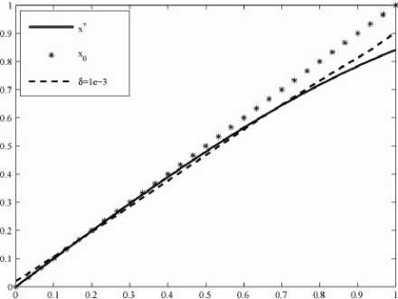
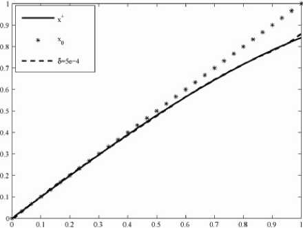
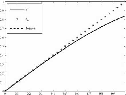
H C k,x)., (t)( hk, hk) H

|c2(t,hk)| < (M2+a+L II y⁵-F(xo^S) II ) HM²

=:^7 H hk H 2,(48)

|b2(t,hk)| < LM H hk H HM3,(49)

L2

|a2(t,hk)| < -y h. 4 : a2 H hk H 4.(50)

Altogether this yields

Ф1(0)- Ф1(1) < ~ HhkH²+X HhkH³+^r HMI⁴

The minimal value of J_o(xn+,, x_n⁶)= ф1(1) is usually unknown, but θmin,k , defined in (45), can be computable. In the case of H h_kH <1 we find

φ1(0)- θmin,k ≤ φ1(0)- φ1(1)

< (M²+a+L H y^s-F(xo^S) H ) H hk H²

+ lm H hk H 3+L4 H hk H⁴

< (M²+a+L H y^s-F(xo^S) H

+ LM+L )HMI²-                 (51)

Thus it follows by using () for H h_kH <1 that

<-VJa(x^k, X_n^$, hk)) > Х(ф1(0)- 0_mln,k)

= /J.l„.(x .. X„^S)- 0m_m,k).

In the case of HhkH>1 we get from ()

-Vj_i;(\   xn⁶, hk)) >Ya.

Inserting the above estimates for <-Vj„(xn.., x_n⁶, h_k)) in

(42) shows that вк<в₀, and, by proposition , the new iterate is therefore closer to x^δn+1 than the old one.

Let

κ1:=Lr(α)+M,

rδ:=

H y^s-F(x₀⁶) Hα

,α)) ,

κ²3:=α²(r²(α)+(r^δ)²),

K2:= H y^s-F(x0⁶) H ²+Mr(a)+Lr(a)².

Theorem 10 Let the assumptions of theorem 5 hold, Kr(a)(x^s+1) be defined as in (36), xn⁶,0=xn⁶^ K.„. i\..i. and {x ^δn,k }k∈N be the iterates of steepest descent for the modified Tikhonov functional with вк chosen according to proposition 9. Then, there exists a constant

K:=2κ21 +2Lκ2+2α+6κ1κ*+3L2κ3,(52)

κ*:=2(κ1κ2+κ3),(53)

such that the second derivative of

0k(t):= Ja(xSx-tVJa(xSx, xn6), xn6) tG[0,1](54)

is bounded by

10''(t)| < K!|Vj_a(4 xn⁶) H 2.

Proof. According to the choice вк all iterates are in Kr(a)(x^s+1). The definition of Vj_a(xn__k, xn⁶) shows that H VJa(x,. xn⁶) H is bounded in Kr(a)(x^s+1) by a constant κ* defined in (53), we have

H VJa(x^S,k, x )

< 2( H F'(xSx) H H y^s- F'(xSx) H +a H xn,- x^sn H ).

and

H F'(xSx) H < H F'(xSx)- F'(xS+1) H + H F'(xS+1) H

< L H x+1n -xS,k H

H y^s- F'(xSx) H < H y^s- F'(xS+1) H H F'(xS+1) - F'(xSx) H

< H y^s- F'(x^s0) H + H F'(xn+1) H H xs+1 -xn, H +L H xs+1 -xs,k H²

< H ys- F'(xs0) H +M r(a)+ L r(a)2=K2,(56)

a2Hxsn,k- xsn H2 < a2 (Hxsn,k- xsn+1  H2+ H  xsn+1- xsn

≤ α 2 (r(α)2+( rδ)2) = κ23 .(57)

Thus

H VJa(xs,k, xn) H

holds for all k. Defining C k,x_n+1 (t)( hk, hk) as in (47) with hk replaced by -Vja(x^sn,k, xn ) and setting

C k,xn+, (t)( - V Ja(x^s,k, xn ), - V Ja(x^s,k, xn ))

=j0F"(x^s,k- tTVJa(x^s,k, xn))( -VJa(x^s,k, xn), -VJa^, xn ))dT we find

θ^'k^'(t)

= 2 H F'(xs,) VJa(xs„ xn) H -2 <y^s- F(xn._k),

F''(x^s,k-t V Ja(x^s,k, xn⁶))(- VJa(x^s,k, xn ),- V Ja(x^, xn⁶)) ) +2a H VJa(x^s,k, xn) H²

• - 4t <F'(xs,k) VJa(xs,k, xn), "C k,_x.-, (t)(- VJa(xs„ xn),

• -    Vja(x^sn,k, xn )))

• - 2t <F'(xs,k) VJa(xs,k, xn), F"(xs,k-tVJa(xs„ xn))

• • (- VJa(x^s,k, xn⁶),- VJa(x^s,k, xn⁶)))

+2t²<F''(x^s,k-tVJa(x^s,k, xn⁶))(- VJa(x^s,k, xn⁶),- VJa(x^s,k, xn⁶)), C k,_x.), (t) (- VJa(x^s„ xn⁶),- VJa(x^s„ xn⁶)))

+2t2 H "C   k,xL (t) (- VJa(xs,k, xn),- VJa(xs,k, xn)) H 2.

The norm of Ck,xn„ (t) (- Vji;(x .. xn),- Vji;(x .. xn)) and C   k,xn„  (t)( -VJa(xs,k, xn6), -VJa(xs,k, xn6)) can be estimated similarly C k,xδn+1 (t)( hk, hk):

H C k,_xn„ (t) (- VJa(x^s,k, xn),- VJa(x^s,k, xn)) H

• <2 H Vja(xs,k, xn⁶)H 2.

HI C k,_xn+, (t)( - V Ja(x^s,k, xn ), - V Ja(x^s,k, xn )) HI

• < L H VJa(xs„ xn) H 2.

Using the above-given estimates, we can finally estimate

10k(t) | for t G[0,1] by

10k(t) | < (2k1 +2LK2+2a) HVj_a(xn_k, xn) H²

+ 6tK1L H Vj_a(x‘_t, xn) H ³

+ 3t²L²H VJa(xs„ xn) H ⁴

≤ (2κ²1 +2Lκ2+2α+6κ1κ*L+3L²(κ*)²)

•HVj_a(xn„ xn) H²

= KHVja(x^sn,k, xn )H².                           (59)

Now all ingredients for the final convergence proof of the steepest descent method have been collected:

Theorem 11 Let the assumptions of theorem 5 hold, Кг(а)(хП+1) be defined as in (36), xn50=xn5 ^ K. ,ix.. ) and {x δn,k }k∈N be the iterates of steepest descent for the modified Tikhonov functional with вк chosen such that proposition 4 and вk

where K is defined as in (52). Then { x^δn,k }k∈N converges to a global minimizer of J_a(x, x_n⁵):

lim xnk= x   arg min Ja(x, xn⁵)

k→∞             x

Proof. According to the choice вк and x_n⁵₀e K_r(_a>( x_n+1), we have

X_n^S_kEKr(a)( xn+i) kEN.

The sequence {xn5k } is monotonously decreasing and bounded from below, thus there exists J0, s.t J„(xn.„ x., )J for k^». First we will show that вк are bounded from below в, вк - в for all k.

By the definition (33), we have

Ok(t) - 0k(0) = -1 iVJa(x=_k, xn⁵) I ² + t- 0k( t ) 0< t

According to theorem , |Ok(t)| I VJa(xn,k, xn⁵) I 2. Without loss of generality we can assume K≥1. It follows for 0 < t ≤ 1

Ok(t) - 0k(0) < -1 IIVJaKk, xn⁵) I ²

+ 2 K|VJa(x^k, xn⁵) I 2

= (-t+2 K) U, X„^S)|2.        (61)

If we set esp. t = _K ≤ 1,then

0k(K ) - 0k(0) < - 2K IIVJaKk, xn⁵) I 2< 0.

With the definition of θmin,k in (), we find

2K II VJa(x^,k, xn⁵) I ²<0k(0)-0k(K )<0k(0)- 0_min,k

0k(0)- 0mm,k n,,

I VJa(x^k, xn5) I 2 □Sn )I ) - 2K.

2) and from (58) follows

I VJa(x=k, xn5) I □n    ) I ) -"K* .

Inserting (62), (63) in (60) yields вk-min{ "К* ,2^K ,]K ,1}=:в.(64)

Next, we show V Ja(x n,k , x n5 ) ^0 for k^0 by contradiction. Let us suppose  V Ja(xn_k, xn5) does not converge to zero. Then there exists ε0>0 s.t. for every N0∈N exists k > N0 with

I VJaix .. xn⁵) I -Eg.                         (65)

Because J_a(x⁵,k, x_n⁵)= 0_k(0) converge monotonously from above to J⁰,, we can moreover assume that

|0k(0)- J⁰, |<4 £2 <4 £0 .

holds for k large enough. Setting t=вk

Ok(вk) - 0k(0) < вк (-1+^ )IVJa(xnk, xn⁵) I ²

• <    - I   V._Ux .. xn⁵)I²< -^в £0

or

Ja(x=_k+1, xn⁵) - J0. = Ok(вk) - J0.

• <    0k(0)- Ja"^ £2

pk 2 р^ 2     pk ²

≤ 4 ε0 - 2 ε0 = - 4 ε0 < 0, which is a contradiction to V Ja(x 5Л, xn5)J,. As a consequence, VJ„(xn„, xn5) converges to zero. Now by the definition of hkin (37), we finally get by using (43) ya I hk I 2< (-VJa(x5,k, xn5), hk)

• < I VJa(x⁵,k, xn⁵) II hk I ^0, and

x . >x .. for I hk I ^0.

• VI. The Iigra Algorithm

Theorem 12 For the nonlinear implicit iterative method, so long as x₀⁵and a is chosen by

• (i)    I xo⁵-x⁺I < ^(2T-L^)a2^-2Ta0^-T 0) ;

2τ( +η+ )α²0 α^τ

• (ii)    1-L I y^$-F(xg⁸) I > Y > 0;

• (iii)    a - min{a0M²aJ|KL(1+^2 ) I y5-F(x0^S) I , (3ⁱ^2^)LM«y‘-F(xaI)f_l;

τ+ 3τ2-2τ

• (iv)    α0 >    _2τ-2    ,

then, the minima x δn+1 of every functional Jα(x, xn ), n=0,1,…can be given by steepest descent method. The steepest descent method is convergent as xn5 is chosen as iterative value for calculating x δn+1 . When stopping iterative number is determined by discrepancy principle, we have xδn(δ)→x+   δ→0.

Proof. The condition (ii) assures theorem holds, the condition (i), (iii) and (iv) assure theorem holds and the condition (iii) assures rδ≤r(α). Therefore, we can always get xδn ∈Krδ( xδn+1)∈Kr(α)( xδn+1)

with x^δn+1 ∈Kr^δ( x^δn ). The following conclusion can be gotten by theorem and induction.

As mentioned earlier, the IIGRA algorithm is a combination of the steepest descent method for the minimization of the modified Tikhonov functional and an optimization routine for finding a regularization parameter α such that Morozov’s discrepancy principle[1] holds. The algorithm is defined as follows:

Algorithm 13 IIGRA step(1) choose x05 and a satisfied theorem 7, give т > 1 and ε > 0, let n=0;

step(2) let k=0, x⁸n,k = x_n^s;

Figure 1. The numerical effect figure with δ=1e-2.

step(3) calculate VJ_a(x⁸+i,k, x_n^s);

step(4) if II VJa(x⁸+_Lk, x_n^s) || < e, goto step(6);

step(5) choose вк by theorem 6 and calculate

• x n*+t = x n,k+e^kVJa(x .. Xn‘), k=k+1, goto step(3);

step(6) Xn^S+i= x ;

step(7) if II y⁵-F(x⁸+i) II < t8, stop, otherwise let n=n+1 and goto step(2).

• V. Two Numerical Experiments

Within this section we will give two practical relevant examples that meet the requirements of the IIGRA algorithm.

Example 1: nonlinear Hammerstein integral equation F(x)s:=J0ф(x(s))ds=y⁵ D(F):=H¹[0,1]→L²[0,1]

Figure 2. The numerical effect figure with δ=1e-3.

where assumption 1 are satisfied[2].

The first Fréchet derivate and transposition of operator F have the following form:

(F'(x)h)(t) = ∫^t0 φ' (x(s))h(s)ds,

(F'(x)^*h)(t) = B^-1[φ'(x(s)) ∫s¹h(t)dt. ] where

(B^-1z)(s) = ∫¹0k(s,t)z(t)dt.

cosh(1-s)cosh(t)

sinh(1)         - k(s,t): = '

cosh(1-t)cosh(s) sinh(1)

t > s

Therefore, the iterative scheme of IIGRA is:

Figure 3. The numerical effect figure with δ=5e-4.

B^-1[φ'(x(s)) ∫s¹h(t)dt. ]

= ∫¹0 k(s,t) φ'(x(t))[ ∫t¹ y^δ(ξ)dξ-∫t¹ ∫^ξ0 φ(x(η))dηdξ]dt.

Set φ(x)=e^x, then true solution x⁺=sin(t). We use IIGRA algorithm solve example 1 in different error level δ with iteration initial value x0(t)=t, τ=1.1, ε=1e-5, α=50.

Table I shows the calculation results of example 1 where  eo= II a » -a+ II l2,  en= I a П   -a+ II L2and n(8)  is iteration numbers. We can see that absolute error en decreases with δ minishing. This is consistent of the conclusion in theorem 11. Fig.1-Fig.4 give the figures of x0, x+ and xns in different 8.

TABLE I.

THE NUMERICAL RESULTS OF EXAMPLE 1 IN DIFFERENT δ

δ	n(δ)	e0	en	en/ e0
1e-2	93	6.059e-2	1.808e-2	0.289
5e-3	118	6.059e-2	1.131e-2	0.187
1e-3	233	6.059e-2	3.720e-3	6.159e-2
5e-4	78	6.059e-2	3.281e-3	5.415e-2
1e-5	72	6.059e-2	2.001e-3	3.303e-2
5e-6	84	6.059e-2	9.804e-4	1.618e-2
1e-7	84	6.059e-2	1.205e-4	1.989e-3
5e-8	84	6.059e-2	5.356e-5	8.840e-4

Figure 4. The numerical effect figure with δ=5e-8.

Example 2: parameter identification a(x) in BVP

-(aux)x=-e^x

u(0)=1

u(1)=e where a(x)∈H1[0,1] and assumption 1 are satisfied[5].

Indeed, example 2 defines a nonlinear operator F:

F(a)=u(a)

D(F)={H1[0,1]| a ≥ a* > 0}.

TABLE II.

THE NUMERICAL RESULTS OF EXAMPLE 2 IN DIFFERENT a^δ0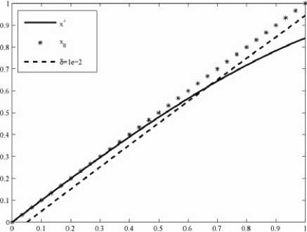

aδ0 n(δ) e0 en en/ e0 0.7 67 0.298 0.138 0.463 3 79 1.98 1.243 0.628 7 332 5.953 3.992 0.671 1+0.05sin(10πt) 44 3.532e-2 5.421e-3 0.153 1+0.1sin(10πt) 49 7.067e-2 8.564e-3 0.121 1+0.3sin(10πt) 58 0.212 8.772e-2 0.413 operator in numerical implementation. Results of examples show its convergence and effectivity. In the next work, we will focus on weakening the restrictions on the property of nonlinear operator.