Numerical Oscillations of Runge-Kutta Methods for Differential Equations with Piecewise Constant Arguments of Alternately Advanced and Retarded Type

Published Online June 2011 in MECS

The theory of the oscillation is one of the most interesting topics for applications. In recent years, the oscillations of difference equations [1,2], dynamic equations [3,4] and delay differential equations [5-8] have been studied and developed by many authors. Among these investigations, oscillations of solutions of differential equations with piecewise constant arguments (EPCA) have also been the subject of many recent investigations [9-12].

It is well known that studies of EPCA were motivated by the fact that they represent a hybrid of continuous and discrete dynamical systems and combine the properties of both the differential and difference equations. These equations play an important role in numerous applications [13,14]. And the theory of EPCA was developed intensively in the last few decades, such as [15-19]. For a brief summary of the theory, the reader is referred to the book by Wiener [20].

Recently, some important results on the properties of the numerical solutions of EPCA have been obtained, such as the stability [21-24] and the oscillations [25,26]. In [25,26], the authors considered the oscillations of numerical solutions in 9 -methods and Runge-Kutta methods for the same equation, respectively. Our paper contains an attempt to enrich the gap by considering oscillations of the Runge-Kutta methods for a more complicated equation and discussing the relationship between stability and oscillations.

In the present work, we shall consider the equation

x'(t) = ax(t) + bx([t + 0.5]), t > 0

• <                                                                 . (1)

_ x(0) = x0,

where a , b , x ₀ are real constants and [.] denotes the greatest integer function. Since the argument deviation of (1) is positive in [ n , n + 0.5) and negative in [ n + 0.5, n + 1) , (1) is said to be of alternately advanced and retarded type. We aim to investigate the oscillations of the numerical solutions in the Runge-Kutta methods for (1) , and get some relationships between stability and oscillations.

The paper is organized in the following manner. In the next section, we give known definitions and results that will be needed further. Section 3 discusses the oscillations and non-oscillations of the numerical solution. We will prove that the oscillations of the analytic solution are preserved by the Runge-Kutta methods. In Section 4, we will obtain the relationship between stability and oscillations. Appropriate numerical examples are given to illustrate our results in Section 5.

• II.    P RELIMINARIES

In this section, we shall introduce some definitions and theorems.

Definition 1 [20] A solution of (1) on [0, да ) is a function x ( t ) satisfies the conditions:

• •     x ( t ) is continuous on [0, да) ;

• •    The derivative x '( t ) exists at each point t G [0, да ) , with the possible exception of the points t = n + 0.5, n = 0,1,2, L , where onesided derivatives exist,

• •    Eq. (1) is satisfied on [0,0.5) and each interval

[n - 0.5, n + 0.5) for n = 1,2,L .

The solution of (1) is given in the following theorem.

Theorem 1[20] If b *

a a/2      , e -1

then (1) has on [0, да) a unique solution x(t) = to(r(t))2[*+0.5]x0 , where

® ( t ) = e a + ( e a - 1 ) a 1 b ,

r ( t ) = t - [ t + 0.5],

.   ^ (1/2)

^               •

^ ( - 1/2)

Definition 2 A non-trivial solution of (1) is said to be oscillatory if there exists a sequence {tk }^=1 such that tk ^ да as k ^ да and x(tk)x(tk-1) < 0; otherwise it is called non-oscillatory. We say (1) is oscillatory if all the non-trivial solutions of (1) are oscillatory; we say (1) is non-oscillatory if all the non-trivial solutions of (1) are non-oscillatory.

In [20,27], the authors establish the following oscillation results.

Theorem 2 If any of the conditions where x = ha and S(x) = 1 + xBT (I - xA )1 e is the stability function of the method. From [24], we know that the Runge-Kutta methods preserve the original order for (1).

We assume that S(x) * 0 and b *

a

.

S ( x ) ^m - 1

Then it follows from (3) that xz = Q(1)x0,   1 e M(0), x2km = Px2(k-1)m,    k > 1                 (4)

^x 2 km + 1 = Q ( 1 ) x 2 km ,     1 e M ( k ),           (5)

where

Q ( 1 ) = S ( x ) ¹ + b ( S ( x ) ¹ -1 ) ,   - m <  1 <  m ,

M ( k ) = { 0,1, L , m -1 } , for k = 0 ,

M ( k ) = { - m , - m + 1, L , m - 2, m -1 } , for k > 1 . and

Q ( m ) _.

Q ^{( -} m )

and

b >

a a/2

e - 1

b <

ae

a /2

a /2

e - 1

holds true, then (1) is oscillatory. Eq. (1) is non-oscillatory if and only if condition

ae

a /2

a /2

e^a  - 1

< b <

a a/2

e^a - 1

is satisfied.

From Definition 2, we can see that if a solution x ( t ) of (1) is non-oscillatory and continuous, then it must be eventually positive or negative. That is, there exists a T e R such that x ( t ) >  0 or X ( t ) <  0 for t >  T .

• III.    O SCILLATION ANALYSIS

• A. Runge-Kutta methods

Similar to [24], let h — 1/ (2 m ), the v - stage Runge-Kutta        methods         ( A , B , C )         with

A = ( a ) , B = ( b 1 , b 2 , L , b v ) ^T          and

X j / vxv

C = ( c 1 ,c ₂ , L , c _v ) ^T applied to (1) yield the recurrence relation

x.,^,_ш = S ( x ) x., ^,+ — (S ( x ) - 1) x,, ,      (3)

2 km + 1 + 1       x / 2 km + 1       \ v л ) 2 km ,        ^{x 7}

a

B. Numerical oscillations and non-oscillations

For any given Runge-Kutta methods, we assume that 5 1 < 0 <  5 2 such that

0 <  S ( x ) < 1, for 5 1 <  x < 0, and

1 <  S ( x ) < да, for 0 <  x <  5 2 , which implies

0 <  S C ^x )—1 < да, for 5 1 <  x <  5 2 . x

For the sake of simplicity, we omit the definition of oscillations of (5) (see [26]). The following theorem gives the relationship of the non-oscillations between { x n } and

. 2 km

Theorem 3 { x n } and { x ₂ km } are given by (5) and (4), respectively, then { x_n } is non-oscillatory if and only if { x _{2 km} } is non-oscillatory.

Proof: The necessity is obvious. In the following, we prove the sufficiency. If { x ₂ km } is non-oscillatory, without loss of generality, we assume that { x _{2 km} } is an eventually negative solution of (4), that is, there exists a k_n e R such that x_n, < 0 for k >  k_n . We will prove 0                         2 km                     0

x2km+1 < 0 for all k > k0 +1 and 1 e M(k). Suppose b < 0, if a < 0 , then 0 < S(x) < 1 and S(x)m < S (x)1, hence x 2 km+1 =f S ( x )1 + b ( S ( x )1 - 1)1x 2 km

I a у

• <| S ( x ) ^m + b ( S ( x ) ^m —1 ) | I a^x v

• = x 2 km + m < ⁰’

If a > 0 , then 1 <  S ( x ) < да and S ( x ) so

x 2 km

— I

^m <  S ( x ) ^{— 1} ,

^{S (} x ) x 2 km ₊ 1

x 2 km

x 2 km

= S ( x ) m x 2 km + m < 0.

Therefore x ₂ km ₊ l < 0 . The proof is complete.

By Theorem 3, we get the following corollary.

Corollary 1 { x n } and { x. respectively, then { x n } i { x 2 km } is oscillatory.

Set

:2 km } are given by (5) and (4), is oscillatory if and only if

a

^A 1 =   a /2

e

A 2 =

ae e a /2

a /2

— 1’

A; ( m ) =---- a ----,

S ( x ) ^m — 1

aS ( x ) ^m

• A, ( m ) =--,

• ²         S ( x ) ^m — 1

then we have

Lemma 1

(i) A 1 1 ( m )

a > 0 or e^x

and А ₂

>A 2 ( m ) if e x >  S ( x )

for

(ii) A , > A 1 ( m ) a > 0 or e^x

< S ( x ) for a <  0;

or А 2 ₂( m ) if e^x <  S ( x ) >  S ( x ) for a <  0;

for

(iii)   A 1 ( m ) ^ A 1 as h ^ 0 and A ₂ ( m ) ^ A ₂

h ^ 0 .

Proof: (i) If a > 0 and e^x >  S ( x ) , then

as

e a /2

which is equivalent to

> S ( x ) ^m ,

e a /2

- <---------,

1 S ( x ) ^m — 1

so we have A 1 < A 1 ( m ) .

By (6), we also have

1 + -71— a/2

e — 1

< 1 +---- ¹

S ( x ) ^m

— 1

that is

e a /2

a /2

e which is equivalent to aea/2

<

S ( x ) ^m

— 1    S ( x ) ^m

— 1’

e a /2

- >

aS ( x ) ^m

S ( x ) ^m — 1’

hence A 2 > A 2 ( m ) . With similar process, the other cases can be proved. This completes the proof.

Theorem 4 Eq. (4) is oscillatory if and only if b > A 1 ( m ) or b < A 2 ( m ) ; (4) is non-oscillatory if and only if A ₂ ( m ) <  b < A 1 ( m ) .

Proof: We can get this result from the fact that (4) is oscillatory if and only if the corresponding characteristic equation has no positive roots.

Definition 3 [26] We say the Runge-Kutta methods preserve the oscillations of (1) if (1) oscillates then there is a h 0 > 0 such that (5) oscillates for h <  h 0 . Similarly, we say the Runge-Kutta methods preserve the nonoscillations of (1) if (1) non-oscillates then there is a h ₀ > 0 such that (5) non-oscillates for h <  h ₀ .

Combining Theorems 2, 3, 4 and Corollary 1, we obtain

• Theorem 5

• (i)    The Runge-Kutta methods preserve the oscillations of (1) if and only if A 1 > A 1 ( m ) or A 2 < A ₂( m ) ;

• (ii)    The Runge-Kutta methods preserve the nonoscillations of (1) if and only if A ₁ < A ₁ ( m ) and A ₂ > A ₂( m ) .

Before giving the conditions that the Runge-Kutta methods preserve oscillations and non-oscillations of (1), we introduce the following corollary.

Corollary 2 [21,22] Suppose S ( z ) = ф( z )/ ^ ( z ) (where ф(z ), ^ ( z ) are polynomials) is the ( r , 5 ) -Pad e approximation to e^z . Then

• a)    S ( x ) <  e^x if and only if 5 is even for all x > 0 ,

• b)    S ( x ) >  e^x if and only if 5 is odd for all 0 <  x <  ^ ,

• c)    S ( x ) >  e^x if and only if r is even for all x < 0 ,

• d)    S ( x ) <  e^x if and only if r is odd for all 7 7 <  x < 0 ,

where ^ is a real zero of y_s ( z ) and n is a real zero of Ф г ^{( z} ) ’

Applying Theorem 5, Lemma 1 and Corollary 2, we can obtain the following theorems.

Theorem 6 Suppose S ( z ) is the ( r , 5 ) -Pad e approximation to e^z , the Runge-Kutta methods preserve oscillations of (1) if any of the following conditions is satisfied:

• (i)    a > 0, h <  h ₁ and 5 is odd,

• (ii)    a < 0, h <  h ₂ and r is odd, where h 1 = — £ 1 / a , h ₂ = — 5 2 1 a .

Theorem 7 Suppose S ( z ) is the ( r , 5 ) -Pad e approximation to e^z , the Runge-Kutta methods preserve non-oscillations of (1) if any of the following conditions is satisfied:

(i) a > 0, h <  h ₁ and 5 is even,

(ii) a < 0, h <  h 2 and r is even, where h 1 = — 5 1 / a , h 2 = —5 2 / a.

Tables 1-2 visually illustrate Theorems 6 and 7 respectively, where "  — " denotes no limitation to parameters. And we give the conditions that the A -stable higher order Runge-Kutta methods preserve oscillations and non-oscillations of (1) (see Tables 3-4).

TABLE 1

PRESERVATION OF OSCILLATIONS

a	h	r	s
a > 0	h <  h 1		odd
a < 0	h <  h 2	odd

Let

TABLE 2

PRESERVATION OF NON-OSCILLATIONS

a	h	r	s
a > 0	h <  h 1		even
a < 0	h <  h 2	even

TABLE 3

PRESERVATION OF OSCILLATIONS FOR HIGHER ORDER

RUNGE-KUTTA METHODS

	Gauss-Legendre	Radau IA, IIA	Lobatto IIIA, IIIB	Lobatto IIIC
( r , s )	( y , y )	( u — 1, u )	( u — 1, u — 1)	( u — 2, u )
a > 0	u is odd	u is odd	u is even	u is odd
a < 0	u is odd	u is even	u is even	u is odd

TABLE 4

PRESERVATION OF NON-OSCILLATIONS FOR HIGHER ORDER

RUNGE-KUTTA METHODS

	Gauss-Legendre	Radau IA, IIA	Lobatto IIIA, IIIB	Lobatto IIIC
( r , s )	( u , u )	( u — 1, u )	( u — 1, u — 1)	( u — 2, u )
a > 0	u is even	u is even	u is odd	u is even
a < 0	u is even	u is odd	u is odd	u is even

IV. R ELATIONSHIP BETWEEN STABILITY AND OSCILLATIONS

Theorem 8 [20] The solution of (1) is asymptotically stable (the solution X ( t ) ^ 0 as t ^ да ) for any given x ₀ , if and only if

a (ea +1)    ,

--75----7 < b < — a, for a > 0,

(ea/2 — 1)2

,           ,      a (ea +1)

b < — a or b > --75---- 7 , for a <  0,     (7)

(ea/2 — 1)2

b <  0 , for a = 0.

Theorem 9 [24] The numerical solution of (1) is asymptotically stable ( X ( t ) ^ 0 as t ^ да ) if and only if

—

a (S (x )2 m +1)   ,

------------7- < b < — a, for a > 0,

(S (x) m — 1)2

,          ,     a (S (x )2 m +1)

b < — a or b > --—, for a <  0 , (8)

(S (x) m — 1)2

b <  0 , for a = 0.

A 3

a ( e^a + 1 ) ^,

and

A 3 ( m ) =

a (S (x )2 m +1) (S(x)m — 1)2 , by Theorems 2, 4, 8 and 9 we get the following theorems.

Theorem 10 For a >  0 , the analytic solution of (1) is

• a)    oscillatory and unstable if b £ ( —да , A 3 ) or b £ ( A 1 , +да ) ;

• b)    oscillatory and asymptotically stable if b £ ( A 3 , A ₂) ;

• c)    non-oscillatory and asymptotically stable if b £ ( A ₂, — a ) ;

• d)    non-oscillatory and unstable if b £ ( — a , A ₁ ) .

for a < 0 , the analytic solution of (1) is

• a)    oscillatory and asymptotically stable if b £ ( —да , A ₂) or b £ ( A 3 , +да ) ;

• b)    non-oscillatory and asymptotically stable if b £ ( A ₂, — a ) ;

• c)    non-oscillatory and unstable if b £ ( — a , A ₁ ) ;

• d)    oscillatory and unstable if b £ ( A ₁ , A ₃ ) .

Theorem 10 For a > 0 , the numerical solution of (1) is a) oscillatory and unstable if b £ ( —да , A 3 ( m )) or b £ ( A 1 ( m ), +да ) ;

• b)    oscillatory and asymptotically stable if b £ ( A 3 ( m ), A ₂( m )) ;

• c)    non-oscillatory and asymptotically stable if b £ ( A ₂( m ), — a ) ;

• d)    non-oscillatory and unstable if b £ ( — a , A ₁ ( m )) .

for a < 0 , the numerical solution of Eq. (1) is

• a)    oscillatory and asymptotically stable if b £ ( —да , A ₂ ( m )) or b £ ( A 3 ( m ), +да ) ;

• b)    non-oscillatory and asymptotically stable if b £ ( A ₂( m ), — a ) ;

• c)    non-oscillatory and unstable if b £ ( — a , A ₁ ( m )) ;

  d) oscillatory and unstable if b £ ( A 1 ( m ), A 3 ( m )) .

  
  

  V. N UMERICAL EXPERIMENTS

  
  

  In order to give a numerical illustration to the main

  
  

  theorems in the paper, we consider the following equations:

  J x '( t ) = x ( t ) - 10 x ([ t + 0.5]),     t >  0

  | x (0) = 1,

  J x '( t ) = - 2 x ( t ) - 5 x ([ t + 0.5]),     t >  0

  | x (0) = 1,

  J x '( t ) = 3 x ( t ) - 2 x ([ t + 0.5]), t >  0

  | x (0) = 1,

  J x '( t ) = - x ( t ) - x ([ t + 0.5]), t >  0

  | x (0) = 1,

  
  

  four

  
  

  0.5

  -0.5

  -1

  -1.5

  

  15         20

  25        30

  
  

  0.5

  -0.5

  -1

  -1.5

  

  15         20

  25        30

  
  

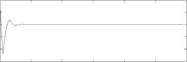
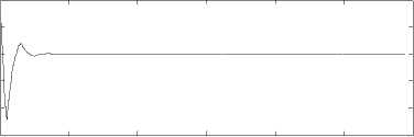
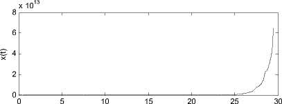
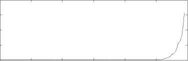
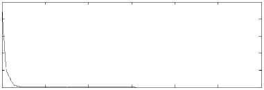
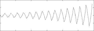
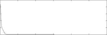
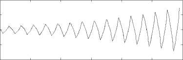
  According to Theorem 2, the analytic solutions of (9) and (10) are oscillatory, the analytic solutions of (11) and (12) are non-oscillatory. In Figs. 1-4, we draw the figures of the analytic solutions and the numerical solutions using 1-Gauss-Legendre method, 2-Radau IA method and 2-Lobatto IIIC method. From these figures, we can see that the numerical solutions of (9) and (10) are oscillatory, the numerical solutions of (11) and (12) are non-oscillatory, which are in agreement with Theorems 6 and 7.

  
  

  Figure 2. The analytic solution and the numerical solution for (10) by 2-Radau IA method with m=50

  
  
  

  In Fig. 1, let m = 50, so A 1 B 1.5415, A ₂ B - 2.5415, A ₃ B - 8.8354, A 1 ( m ) B 1.5415, A ₂( m ) B - 2.5415 and

  
  

  x 10¹³

  

  0          5         10         15         20         25         30

  Figure 3. The analytic solution and the numerical solution for (11) by 2-

  Lobatto IIIC method with m=50

  
  

  A ₃( m ) B - 8.8353, Obviously, b = - 10 £ ( -^ , A 3 ) and b = - 10 £ ( -^ , A 3 ( m )). Therefore, the analytic solutions and the numerical solutions of (9) are both oscillatory and unstable according to Theorems 10 and 11, which are in agreement with Fig. 1. For (10)-(12), we can verify the consistency in the same way (see Figs. 2-4).

  All these numerical examples confirm our theoretical findings.

  
  
  
  
  
  

  0.8

  0.2

  0.6

  0.4

  
  
  
  

  -20

  -40

  0          5         10         15         20         25         30

  
  

  0.8

  0.6

  0.4

  0.2

  

  5         10         15         20         25         30

  Figure 4. The analytic solution and the numerical solution for (12) by 2-Lobatto IIIC method with m=50

  
  

  -20

  -40

  
  
  

  0          5         10         15         20         25         30

  
  

  Figure 1. The analytic solution and the numerical solution for (9) by

  1-Gauss-Legendre method with m=50

  
  

  VI. CONCLUSION S

  In this paper, numerical oscillations of Runge-Kutta methods for one important class of EPCA of alternately advanced and retarded type are discussed. The preservation of oscillations of the Runge-Kutta method

  
  

are obtained and the relationships between the stability and the oscillations are considered for the analytic solution and the numerical solution, respectively. Four numerical examples have shown the correctness of the main result. We will consider the Euler-Maruyama method in the future work.

A CKNOWLEDGMENT

The authors wish to thank Professor Mingzhu Liu for his helpful comments and constructive suggestions. This work was supported by the National Natural Science Foundation of China (No. 51008084), the Natural Science Foundation of Guangdong Province (No. 9451009001002753) and the Youth Foundation of Guangdong University of Technology (No. 092027).