Numerical research of the Barenblatt - Zheltov - Kochina stochastic model

Author: Kadchenko S.I., Soldatova E.A., Zagrebina S.A.
Section: Краткие сообщения
Article in issue: 2 т.9, 2016.
Free access
At present, investigations of Sobolev-type models are actively developing. In the solution of applied problems the results allowing to get their numerical solutions are very significant. In the article the algorithm for numerical solving of the initial boundary value problem is developed. The problem describes the pressure distribution of the homogeneous fluid in the horizontal layer in the circle. The layer is opened by a vertical well of a small radius. In our research we suppose that random disturbing loads have an influence on the fluid. The problem was solved under two assumptions. Firstly, we suppose that an unstable fluid flow is axially symmetric, and secondly, that in initial moment the pressure in the layer is constant. After the process of the discretization we modify the original model to the Cauchy problem for the system of ordinary differential equations. For the numerical solution we use algorithms based on explicit one-step formulas of the Runge - Kutta type with the seventh-order accuracy and with the selection of the integration step. We also use the scheme of the eighth-order accuracy to evaluate the calculation accuracy on each steps of time. According to the results of this control, we choose the time-step. A lot of numerical experiments have shown high numerical efficiency of the algorithm that we use to solve the investigated initial-boundary problem.
Stochastic sobolev type equation, numerical solution, barenblatt - zheltova - kochina model, cauchy problem
Short address: https://sciup.org/147159362
IDR: 147159362 | UDC: 517.9 | DOI: 10.14529/mmp160211
Численное исследование стохастической модели Баренблатта - Желтова - Кочиной
В настоящее время активно развиваются исследования математических моделей соболевского типа. В решении прикладных задач значимыми являются результаты, позволяющие получать их численное решение. В работе разработан алгоритм численного решения начально-краевой задачи описывающей распределение давления однородной жидкости в горизонтальном пласте, который вскрыт вертикальной скважиной малого размера. Предполагается, что на жидкость действуют возмущающие случайные нагрузки, а область исследования представляет собой круг с центром на оси скважины. Задача решалась в предположение, что неустановившееся течение жидкости осесимметричное, а в начальный момент времени давление в пласте постоянное. Проводя дискретизацию, исходная задача для дифференциального уравнения в частных производных, преобразована к задаче Коши для системы обыкновенных дифференциальных уравнений. Для численного решения задачи Коши использовались алгоритмы, основанные на явных одношаговых формулах типа Рунге - Кутты седьмого порядка точности с выбором шага интегрирования. Для оценки контроля точности вычислений на каждом временном шаге использовалась схема восьмого порядка точности. Исходя из результатов этого контроля, выбирался временной шаг. Многочисленные вычислительные эксперименты показали высокую вычислительную эффективности алгоритма решения исследуемой начально-краевой задачи.
Text of the brief report Numerical research of the Barenblatt - Zheltov - Kochina stochastic model
Introduction. Let G C R d be a bounded domain with a boundary dG of class C~. Consider in the cylinder G x R+ the Barenblatt - Zheltova - Kochina equation [1]
( A - A) u t = a A u + f, (!)
with the Dirichlet condition
u ( x,t ) = 0 , ( x,t ) G dG x R+ . (2)
Model (1), (2) simulates the pressure dynamics of the fluid filtered in fractured porous medium with random external influences f [2], processes of moisture transfer in a ground [3] and processes of the solid-to-fluid thermal conductivity in the environment with two temperatures [4]. In equation (1) a and A are real parameters, that characterize the environment; the parameter a G R+, and the parameter A can also take the negative values [5]; the additive component f presents the random external load [2]. Our goal is to find the random process u = u ( x,t ) that satisfies (1), (2) with initial Cauchy condition
u ( x, 0) = u о( x ) . (3)
It must be noted that the problem (1), (2) in corresponding Hilbert spaces can be reduced to the linear stochastic Sobolev type ecpiation
Ldu = Mudt + NdW.
You can find more historical aspects of the stochastic equations theory (including the stochastic Sobolev type equations research), for example, in [6].
-
1. Homogeneous Fluid Filtration. Consider the algorithm of construction of numerical solution to (1), (2). As an example we consider unstable filtration of the homogeneous fluid in the horizontal layer. The layer is opened by a vertical well of a small radius. At the initial moment pressure of fluid in the layer is constant and is equal to p 0. Assume that a random load begins to influence the fluid. Let the domain G C R2 be presented by disk with the radius r 0 and center on the axis of the well. Introduce a polar system of coordinates and assume that the fluid flow is axially symmetric. In this case we can find the fluid pressure in a fissure if we solve the initial-boundary value problem [1]
-
2. Results of the Calculation Experiment. The algorithm for solving of problem (4) that was described in previous paragraph, was implemented in a special program in Maple Math Software. This program gives us an opportunity to conduct numerical experiments that find the values of the pressure in breaches under a specific condition. This condition describes random loads, that have difference influence on the seam consumption. We use the random number generator to choose the constant A E R for function that determines random loads for the seam consumption. Estimates of experiments show that in equation (4) the parameter n for different earth materials take the value between very wide limits П = 10 “ 4 m2 ^ 106 m2, and the coefficient x = 0 , 1 m2/s ^ 1 m2/s.
( A — A r ) p t = a A r p + A sin( wt ) , \p (0 ,t ) | < + to , p ( r о ,t )=0 , p ( r 0) = p о ,
d2 1 d , where Ar = 7— +— —, A E R, A = 1 /n, n Is a specific characteristics of the fractured dr2 rdr ground, a = x/n X is the piezoconductivity coefficient of the fractured ground.
Then we need to modify (4) to the system of ordinary differential ecpiations. So we make a discretization of the domain G. We work 0n a segment [0, r0] with the equally spaced grid rj = (j — 1)hr, j = 1, J, hr = r0/(J — 1), J is the number of discretization points. It is known that the construction of difference approximation for the p-th order derivatives in the j-th discretization point is based on the formula
.p 1 j + jp
(= h pE W- . + O^-) . r i = j - j l
where jljjp) is the amount of points 10 the left (right) from the j-th point in which the derivative is calculated, i is numbers of points that we use in the approximation of the derivative nu = jl + jp + 1 is the amount of points that we use in the derivative approximation, nu < J. After we use the expansion of a function p(r, t) in a Taylor series in the point rj, we can simply receive a system of linear equations to find coefficients apji. Ah have already made a, special progra 111 In Maple Math Software to calculate apji for p E N-order derivative and for j, i = 1, J. This program gives an opportunity to use (5) with difference approximation errors O^h^u p^ during the process of numerical
simulations.
After we have done the discretization of initial-boundary conditions (4) we obtain a Cauchy problem for the system of ordinary differential equations for the function u j ( t ). The system we will write in the matrix form
M
dU ^ = pu ( t ) + w, U (0) = U 0 .
|
( |
1 |
0 |
0 |
• •• 0 А |
u 1( t ) |
|||||
|
b 2 , 1 |
λ - b 2 , 2 |
b 2 , 3 |
. . . b 2 ,J |
u 2( t ) |
||||||
|
Where |
M = |
... |
... . |
.. |
...... , U ( t ) = |
1 1 |
||||
|
b J - 1 , 1 |
b J - 1 , 2 b J - |
1 , 3 .. |
. λ - bJ - 1 ,J |
u |
1 - 1( t ) |
|||||
|
0 |
0 |
0 |
••• 1 |
u |
1J ( t ) / |
|||||
|
u 01 |
1 |
( 1 |
0 |
0 ••• 0 А |
( 0 А |
|||||
|
u 02 |
b 2 , 1 |
b 2 , 2 |
b 2 , 3 . . . b 2 ,J |
A sin( wt ) |
||||||
|
U 0 = |
• • • |
, P = |
... |
... |
... ... ... |
, W |
= |
= |
• • • |
|
|
u 0 J - 1 |
b J - 1 , 1 b |
J - 1 , 2 |
b J - 1 , 3 . . . b J - 1 ,J |
A sin( wt ) |
||||||
|
u 0 J |
0 |
0 |
0 ••• 1 У |
0 |
||||||
Uj is values of pressure in the j-th point of digitalization. If we don’t use the point in derrivativa approximation, then bji = 0, otherwise bji = -2ji +--j. where the first hr2 rj hr index j indicates the number of the point in which we make the derivative approximation and the second index i indicates the number of point, that takes part in the derivative approximation.
It’s easy to show that the determinant of the matrix P is not equal to 0. In rare cases when we set A it may be that the determinant of the matrix M equals to 0. In this case we need to change the amount of points that take part in derivatives approximation. It will change the value of the determinant of the matrix P and consequently change the value of the determinant of matrix M. Therefore, we assume that det(M) = 0.
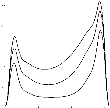
After the invertion of the matrix M from equation (6), we obtain a Cauchy problem for the first-order differential equations in the matrix form dU(t) TT, xx dt- = F(t,U(t))’ 0 where F(t, U(t)) = M-1PPU(t) + W^. For the numerical solution of (7) we use algorithms that are based on explicit one-step formulas of the Runge - Kutta type with the seventh order accuracy [7]: Un +1 = Un + ^ pniki, i=1 13 13 = hFl tn + ah ^n + 52 в^kj, An + 52 в^kj ) • j=1 j=1 ki Where ht is a integration step in Runge - Kutta method, a i = 0, a 2 = 27, a 3 — _, a — —, a^ , ae — —, a? — —, 9 ’ 4 6 ’ 5 12 ’ 6 2 ’7 6 ’ a 8 = X, a 9 = X, 6 3 1 a 10 = 3 ’ a 11 = 1’ a 12 = 0’ a 13 = 1’ 2 1 в2’1 = 27 ’ в3’1 = 36 ’ e 5,1 = 12 ’ e 5,2 = 0’ e 5,3 = 11 1 e 3,2 = — ’ e 4, 1 = 24 ’ e 4,2 = 0’ e 4,3 = ^ ’ 25 25 1 " — 16 ’ в5,4 = 16 ’ в6,1 = 20 ’ в6,2 = в6,3 = 0’ e 6,4 = 4 ’ в6,5 = 5 ’ в 7,1 = β = 125β = 31 e7,6 54 ’ в8,1 300 ’ 25 125 108 ’ в 7,2 = в 7,3 = 0’ в 7,4 = 108 ’ в 7, 5 = в 8,2 = в8,3 = в 8,4 = 0’ в8,5 = 225’ в 8,6 = 13 23 704 e8,7 = 900 ’ в 9,1 = 2’ в 9,2 = в 9, 3 = 0’ в 9’4 = 108 ’ в9’5 = 15 ’ в 9,6 = -27, - 9, -9, 67 91 в 9,7 = 90 ’ в9,8 = 3 ’ в 10,1 = — 108 ’ в 10,5 = — ,-’ в 10,6 = WW’ в 10,7 = 135 54 в 11,1 = 4100 ’ в 11,2 = в 11,3 = 0’ в 11,4 = e 10,2 = e 10,3 = 0’ e 10. ',4 = 108 ’ -60, 341 - 164, в 10,8 = "6’ в 10,9 = - 12, e 11,5 = 1025 ’ e 11, 6 = 82 , 2133 45 45 18 в 11,7 = 4100 ’ в 11,8 = 82 ’ в 11,9 = 164 ’ в 11,10 = — 41 ’ в12,1 205 ’ e 12,2 = e 12, 3 = e 12, 4 = e 11,5 = 0’ в 12,6 = - 41 ’ в 12,7= 205, в 12,8 = - 33 6 41 ’ в 12,9 = 41 ’ в 12,10 = 41 ’ в 12,11 = 0’ в 13,1 = 341 4496 в 13,2 = в 13,3 = 0’ в 13,4 = —164 ’ в13,5 = 1025 ’ в 13,6 = 4100, 82 , 2193 51 33 12 e 13,7 = — 4100 ’ в 13,8 = 82 ’ в 13, 9 = 164 ’ в 13,10 = 41 ’ в 13,11 = 0’ в 13,12 = 1’ 41 34 9 p7,1 = 840 ’ P7,2 = P7,3 = P7,4 = P7’5 = 0’ P7’6 = 105 ’ P7’7 = P7,8 = 35 ’ p 7,9 = P 7,10 = 280’ p 7,11 = 840’ p 7,12 = p 7,13 = 0• When we use explicit methods to solve the stiff problem we would like to note that the integration step is limited not only by calculation accuracy but also by the stability of the numerical method [8]. We can find the local error 5n of the method with the seventh order accuracy by using the next formula [7] 5n = E( P 8 ,i i=1 - P 7 ,i) ki’ where coefficients p8i are equals p 8,1 = p 8,2 = p 7,3 = p 7,4 = p 7,5 = 0’ p 7,6 = ^5’ p 8,7 = p 8,8 = 35’ p 8,9 = p8,10 = 280 p 8,11 = p 8,12 = 0’ p8,13 = 840 • If you would like to evaluate the control of the calculation accuracy you can use the next inequality ll^nll < e. Неге || • || is a norm in RJ, J is the dimension of the matrix column F(t, U(t)), г is the necessary calculation accuracy. In our case 5n = O ht8 . Therefore integration step hac according to accuracy is calculated with the formula [8] ha=qht ■ q=■ In the case q < 1 we need to repeat the calculation that we received at the step ht and use the other step hac. Otherwise we must repeat our calculations on the next interval of time. Fig 1. Dependence of pressure p = p(t* ,r) in a fissure at moments of time t* = 1,27s, t* = 2,61 s, t* = 4s Fig 2. Dependence of pressure p = p(t, r) in fissure on t and r Numerous calculations have shown that the developed algorithm of the solution allows to find the numerical solution of the problem with high computational efficiency.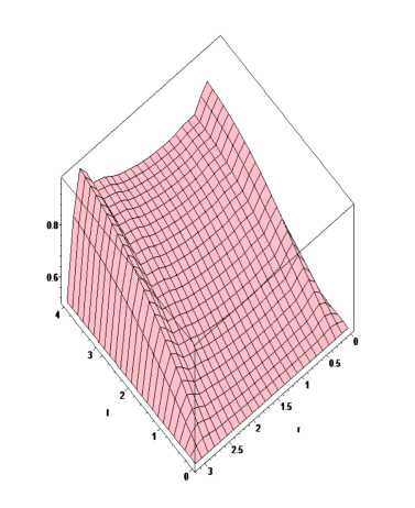
References Numerical research of the Barenblatt - Zheltov - Kochina stochastic model
- Баренблатт, Г.И. Об основных представлениях теории фильтрации в трещиноватых средах/Г.И. Баренблатт, Ю.П. Желтов, И.Н. Кочина//Прикладная математика и механика. -1960. -Т. 24, № 5. -С. 58-73.
- Загребина, С.А. Линейные уравнения соболевского типа с относительно p-ограниченными операторами и аддитивным белым шумом/С.А. Загребина, Е.А. Солдатова//Известия Иркутского гос. ун-та. Серия: Математика. -2013. -Т. 6, № 1. -С. 20-34.
- Hallaire, M. On a Theory of Moisture-Transfer/M. Hallair//Inst. Rech. Agronom. -1964. -№ 3. -pp. 60-72.
- Chen, P.J. On a Theory of Heat Conduction Involving Two Temperatures/P.J. Chen, M.E. Gurtin//Z. Angew. Math. Phys. -1968. -V. 19. -P. 614-627.
- Свиридюк, Г.А. Задача Коши для линейного сингулярного уравнения типа Соболева/Г.А. Свиридюк//Дифференциальные уравнения. -1987. -Т. 23, № 12. -С. 2169-2171.
- Sviridyuk, G.A. The Dynamical Models of Sobolev Type with Showalter -Sidorov Condition and Additive Noise/Sviridyuk G.A., Manakova N.A.//Вестник ЮУрГУ. Серия: Математическое моделирование и программирование. -2014. -Т. 7, № 1. -C. 90-103.
- Новиков, Е.А. Контроль устойчивости метода Фельберга седьмого порядка точности/Е.А. Новиков, Ю.В. Шорников//Вычислительные технологии. -2006. -Т. 11, № 4. -С. 65-72.
- Новиков, Е.А. Разработка алгоритмов переменной структуры для решения жестких задач: дис.. канд. физ.-мат. наук/Е.А. Новиков. -Красноярск, 2014. -123 с.
