Numerical simulation of droplet coalescence in turbulent stream using level set method

Two phase flow are encountered in a wide range of industrial as well as engineering applications, e.g. bubble and droplet dynamics [1], atomization and spray of liquid jet [2], and other multiphase flow systems [3].

Due to the importance of droplet dynamics in most of atomization systems, there is an increased attention being given for the prediction of deformation and disintegration of droplets either numerically, analytically or experimentally. It is well known that the combustion efficiency in diesel engines, gas turbine engines, oil

* Corresponding author. Tel.: +966582351586

burners and liquid rockets is strongly dependent on liquid fuels atomization process [4].

Consequently, atomization process remains a challenging topic of research [5]. Turbulence usually interacts with other atomization mechanisms, such as surface instabilities, ligament formation, stretching and fragmentation to transform large scale coherent liquid structures into small scale droplets. Generally, atomization process that occurs in a turbulent environment usually includes a wide range of time and length scales [6].

The numerical investigations of the atomization process are scarcely due its computational challenges [7]. Although drops seldom occur in isolation, it is essential to understand the behaviour of single and binary droplets before a full knowledge on interacting can be achieved. Disturbances, which cause disintegration of drops, include: rapid acceleration, high shear stresses and turbulent fluctuations.

In turbulent flow fields, the break-up of the droplets is controlled by the pressure fluctuations of a turbulent motion. The hydrodynamic fluctuations of the pressure are caused by velocity changes. As proposed in [8], only the energy associated with eddies with length scales smaller than the droplet diameter is available to case disintegration, however, larger eddies merely transport drops.

Although several papers have recently reported experimental efforts to understand the physics of the droplet deformation, disintegration and its related dynamics in turbulent flow, however, experimental measurements and the observation of dense and small region with high spatial-temporal resolution in such applications have been difficult [9].

More recently, carefully executed simulations in such context can virtually replace experiments. In general, the numerical predictions of turbulent droplet dynamics have been limited in accuracy partly by the performance of three key elements, viz.: development of the computational algorithm, interface tracking methods, and turbulence prediction models.

During the last decade, a variety of computational fluid dynamics techniques have been developed to study turbulent two-phase flow dynamics. A comprehensive review of the numerical models applied for two-phase flow up to 1996 can be found in [10]. More extended review up to 2010 for the atomization process and its related dynamics can be found in [11].

In the numerical simulation of turbulent droplet dynamics, it has been difficult to predict the physical processes occurred due to the requirement of high resolution, especially for high Weber and Reynolds number. The severe resolution required in such simulation is essentially in order to resolve the important role played by surface tension in ligament and drop formation. Consequently, in order to obtain an insight in such dynamics, the numerical treatments of such processes are carried out in a number of sequential steps starting from the investigation of the surface instability that leads to droplet deformation followed by ligament formation and drop separation from a single ligament till the secondary break-up of liquid droplets.

The application of Direct Numerical Simulation (DNS) in two-phase turbulent flow is currently in the primitive stage as it is limited to relatively low Reynolds number and simple geometries [11]. Consequently, resolving all physical processes in such context is not possible. Although Large Eddy Simulation (LES) has been developed to form a bridge between Reynolds-Averaged Navier-Stokes equations (RANS) and DNS [12], there has not been much of an effort to employ LES for modelling turbulent two-phase flow. In most cases, LES can be directly used in turbulent two-phase flow, provided that the fluids interface does not undergo any significant deformation during the evolution. However, the presence of a rapidly changing of the fluids interface has relatively unknown effects on LES. It is possible that the deformation of the interface has a dynamic interaction with both the resolved and modelled turbulence scales in the flow. At the same time, it is also possible that the modelling of turbulent phenomena by LES has consequences in the computation of the interface dynamics.

The fact that a generally applicable model for turbulence in single-phase flows is not yet available compounds the problem for two-phase turbulent flow. However, RANS type turbulence models with the linear eddy-viscosity models (LEVM), which based on Boussinesq assumption, are still standard in many practical engineering applications.

Among several LEVM, the standard (STD) k- turbulence model [13] is still the most widely used in industrial and engineering applications as it represents a good comparison between accuracy and computational efficiency. It was developed; calibrated and validated to cover a wide range of industrial and engineering applications. It is a robust two-equation turbulence model and it yields quite reasonable results in high Reynolds number flow when its restrictions are undertaken. Therefore, the two-equation STD k-model has been the subject of much research in the last years. Therefore, in the present work; the STD k-turbulence model is applied to predict the droplet collision dynamics in turbulent flow regime.

Usually, in the numerical simulation of turbulent two-phase flow, the Navier-Stokes equations are coupled to one of the available tracking methods in order to predict the complex topological changes of the phase interface. Given examples for such tracking methods, Volume-Of-Fluid (VOF) method [14] and Level Set Method (LSM) [15] are the most popular interface capturing methods. Although the VOF method has been widely applied for predicting different complex two-phase flows, it suffers from several numerical problems such as interface reconstruction algorithms and the difficult calculation of the interface curvature [16]. These numerical problems can, in particular, limit the accuracy and the stability of the numerical method adopted for calculation of two-phase flows, especially when the surface tension is included. A comprehensive review for the different VOF methods and their numerical constraints can be found in [17].

In contrast to the VOF methods, the level set methods offer highly robust and accurate numerical technique for capturing the complex topological changes of moving interfaces under complex motions. The basic idea of LSM is the use of a continuous, scalar and implicit function defined over the whole computational domain with its zero value is located on the interface. The LSM divides the domain into grid points that contain the value of the scalar function; therefore, there is an entire family of contours. The interface is then described as a signed distance function at any time and, consequently, the geometric properties of the highly complicated interfaces are calculated directly from level set function. Moreover, the complex topological changes of interfaces such as merging and breaking-up are handled automatically in a quite natural way without any additional procedure. In addition, the extension of the LSM to three-dimensional problems is easy and straightforward.

Referring to the previous discussion, the LSMs have seen tremendously in different CFD-applications of diverse areas, e.g. two-phase flows, turbulent atomization, grid generation and turbulent combustion [18]. However, the LSMs suffer from numerical diffusion which may cause a smoothing out of sharp edges of interface. The level set function is usually evolved by a simple Eulerian scheme and, consequently, the final implementation of LSM does not provide full volume conservation, so highly accurate transport schemes are required. In our previous work [19], a new technique for solving the level set equation has been developed and validated by performing a number of challenge test cases.

In the present paper, a new numerical method on the basis of the control volume approach is developed and validated by performing the well known fluid dynamics problem of Von-Karman Vortex Street over a fixed circular cylinder. Following, the dynamics of two colliding droplets in different flow regimes is predicted and analysed. The complete system of the governing equations and the associated numerical models and boundary conditions are described in details in the following sections.

• 2.    Physical and Mathematical formulation

2.1. Reynolds-Averaged Navier-Stokes Equations

The governing equations for 2D unsteady, isothermal and incompressible turbulent two-phase flow are described in the present section. The level set method is further explained. Consequently, the associated boundary conditions and the numerical algorithms and models applied for solving the appropriate governing equations are also discussed. The computational grid and the control volumes adopted for solving the governing equations are shown in figure 1, considering for example, a single circular droplet exposed to either laminar or turbulent flow. The level set function is described as well.

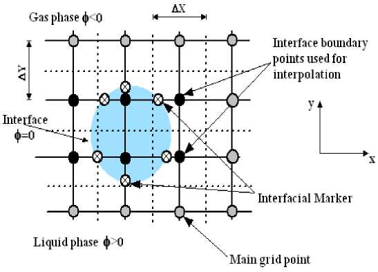
Fig. 1: Computational grid of circular drop and the level set characteristics.

The Reynolds form of the continuity and momentum equations for turbulent two-phase flow, called here RANS equations, at each point of the flow field can be represented by the following equations after neglecting the body force:

∇⋅(ρu)α=0

∂(ρu) +∇⋅(ρuu)+∇p =∇⋅(2µSˆ+ℜˆ ) ∂t                                             t

α

where the subscript α takes the values 1 and 2 and denotes the properties corresponding to the liquid and gas phases, respectively. In the above system of equations, u is the velocity vector, p is the pressure, ρ is the density, µ is the molecular viscosity, S is the strain rate tensor and ℜ is the turbulent stress tensor which are given as:

∂u

S = 0.5(∂ui + uj)

∂x   ∂x

2

ℜ _ij = - ρ u_i ′ u ′ _j = -   ρ k δ _ij + 2 µ _tS_ij

where δ is the Kronecker delta and u ′ u ′ are the average of the velocity fluctuations. The turbulent viscosity is defined as:

µt = ρCµk 2 / ε

The turbulent kinetic energy k and its dissipation rate ε can be estimated by solving the following equations:

∂(ρk)+∇⋅(ρku)=∇⋅(µ+µ/Σ )∇k+2µSˆSˆ-ρε

∂ t                                                                                                               (6)

^{∂ ( ρε )} +∇⋅ ( ρε u ) =∇⋅ ( µ + µ t / Σ ε ) ∇ ε + (2 C 1 ε µ t S ^ˆ S ^ˆ - C 2 ε ρε ) ε / k

∂ t                                                                                                               (7)

The coefficients for the so-called STD k- ε turbulence model are given as follows [13]

C µ = 0.09, Σ k = 1, Σ ε = 1.3, C 1 ε = 1.44, C 2 ε = 1.92

• 2.2.    Level Set Function

The level set method is a class of capturing method where a smooth phase function     is defined over the complete computational domain. The level set function at any given point is taken as the signed normal distance from the interface separates the two fluids with positive on one side (i.e.        ), and negative on the other (i.e.        ). Consequently, the interface is implicitly captured as the zero level set of the level set function, as shown in figure 1. This level set function is updated with the computed velocity field and thus propagating the interface.

The update of the level set function with time can be determined by solving the following transport equation:

∂φ+u ⋅∇φ=0

^{∂ t}                                                                                                             (8)

where u is the velocity vector. Since the interface is captured implicitly, the level set algorithm is capable of capturing the intrinsic geometrical properties of highly complicated interfaces in a quite natural way. Consequently, the normal vector and the curvature of the interface can be defined as:

∇φ n=     ,

I ∇φ,

κ=∇⋅n

The time-stepping procedure for the level set equation is based on the second-order Runge-Kutta method. An important step in the solution algorithm of the level set function is to maintain the level set function as a distance function within the two fluids at all times, especially near the interface region, i.e. the Eikonal equation; ^{∇ φ = 1} should be satisfied in the computational domain. This can be achieved each time step by applying the re-initialization algorithm described in [20] for a specified small number of iterations.

Since the development of the level set method for incompressible two-phase viscous flow [20], a large number of articles on the subject have been published and several types of problems have been tackled with this method; see for instance the cited review [21]. However, the implementation of the level set method in predicting the moving interfaces under turbulent characteristics is indeed very scarce.

• 2.3.    Interfacial Stress Modelling

The jump conditions at the interface separating the two fluids are comprised of the dynamic and kinematic conditions. In the case of two immiscible fluids, taking the projections of the jump conditions in the directions normal and tangential to the interface and considering a constant surface tension, one obtains the following two equations in the normal and tangential directions, respectively:

[p - l^ff (Vu ■ n) ■ n] = OKU

Ц д ( V u ■ n) ■ t + Ц д ( V u ■ t) ■ n] = 0

where O is the surface tension, Ц^ = Ц + Ц is the effective viscosity, к is the curvature of the interface, n and t is the normal and tangential vector to the interface. It is noticed from the above equations that surface tension effects are included in the normal stress balance, while the equality of the shear stress is satisfied in the tangential direction.

The idea of our modelling is straightforward. By introducing a number of so called "Interfacial Markers" on the intersection points of computational grids with the interface, the interfacial stresses are computed at such markers and then it is used to drive the liquid phase through the momentum equations. Moreover, at the position of the interfacial markers, the local curvature is easily estimated by means of a simple interpolation technique. Once the curvature is known, the surface tension force is evaluated.

The present surface tension model ensures that both the pressure calculated within the liquid phase and the surface tension pressure is consistent and dynamically similar, as their effect is determined in the same way. Accordingly, the pressure drop across the interface cancels exactly the surface tension potential at the interface.

For more generality of the present model, see figure 1, it is considered that the interfacial pressure at the pp liquid phase l is determined by evaluating the pressure in the gas phase g and the surface tension pressure, i.e.:

pl = pg + σκ

The pressure values calculated from the above equation are then used as Dirichlet boundary conditions for solving the Poisson equation for the pressure. The above interfacial conditions are known as Laplace’s formula [22] for the surface pressure in case of inviscid incompressible fluids with constant surface tension coefficient. Moreover, in addition to the equality of the dynamically interfacial stresses described above, the kinematic conditions should also be considered. When there is no mass transfer through the interface, the kinematic conditions is satisfied at the moving interface by assuming the continuity of the normal velocity component;

V n _l = V n _g

However, in case of stationary interface, the normal velocity must equal zero. Satisfying the previous interfacial boundary conditions is an important task in the numerical simulation of two-phase flows as the pressure and velocity field inside the liquid phase are caused by the external gas field. Therefore, the exact pressure level inside the liquid phase, which considered as the driving force, should be accurately specified.

• 2.4.    IMLS Numerical Scheme

The present algorithm is based on the implicit fractional step-non iterative method to obtain the velocity and pressure filed in the computational domain. Assuming that the velocity field reaches its final value in two stages; that means

_U n + 1 _{= U} * _{+ U}

whereby, U ^* is an imperfect velocity field based on a guessed pressure field, and U is the corresponding velocity correction. Firstly, the 'starred' velocity will result from the solution of the momentum equations. The second stage is the solution of Poisson equation for the pressure:

∇2p = ρα∇⋅U* c   ∆t

where Δ t is the prescribed time step and p is called the pressure correction. Once this equation is solved in each phase, one gets the appropriate pressure correction and, consequently, the velocity correction is obtained according to the following equation:

U

-

c

∆t

∇ p_c

ρα

This fractional step method described above ensures the proper velocity-pressure coupling for incompressible flow field. However, the accurate solution of the surface pressure occurring at transient fluid interfaces of arbitrary and time dependent topology enables an accurate modelling of two- and three dimensional fluid flows driven by surface forces. Assuming that a square regular mesh is used for the calculation, the curved shape of the interface causes unequal spacing between the interface and some internal grid points, as illustrated in figure 2. In the present work, a linear interpolation is used to assign values of the curvature at the interface from the known internal grid points values.

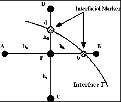
Fig. 2: Calculation of the interphase boundary values.

Referring to figure 2, the interphase boundary value of the curvature can be calculated according to the following relation:

К ^{( ф )} = (1 - f)к_Р ^{( Ф )} + f ^K B ^{( Ф )},     f = ^ф р /^{( ф} р - ^ф )

The calculation of the local curvature at the interfacial markers enables us to calculate the surface tension force, i.e. the surface pressure. Consequently, an approximation of the Poisson equation for pressure at point p can be represented as follows:

P y =

+ p + p + pc + e . ^ha ^{( h}a ^{+ h}b )    ^hb ^{( h}a ^{+ h}b )    ^hc ^{( h}c ^{+ h}d )    ^hd ^{( h}c ^{+ h}d )

where S_p is the source term described in Eq. (15). The above equation can be developed utilizing Taylor-series expansion about the grid point p . It can easily be shown that the above formula is equivalent to that in case of a regular grid formula if the distances h_a = h b = A x, and h_c = h_d = A y . More details about the numerical procedure used to solve the above system of equations can be found in [23].

The above algorithm is applied in a separate way in both phases to obtain the fluid variables in each phase. By using the velocity and pressure values on the gas phase as a boundary conditions defined on the interface, the solution of the liquid phase is carried out. After that, the turbulent equations are solved on both phases simultaneously. The normal velocity at the interface is then used to move the interface using the level set approach and to obtain its topological changes. Consequently, the whole algorithm is repeated until it would reach the statistically steady state condition.

• 3.    Validation

The prediction of the velocity field and vorticity structure for flow around a stationary circular cylinder for a wide range of Reynolds number is an important as well as a challenge benchmark CFD problem. Therefore, such flow represents a canonical problem for validating new approaches in computational fluid dynamics. The formation and shedding of vortices in a cylinder wake could result in periodic fluid forces acting on a circular cylinder. Consequently, the control of vortex shedding from a circular cylinder is an important topic of interest in fluid engineering [24]. Moreover, the prediction of the flow around an immovable cylinder is considered to be a precursor to the flow around a deforming droplet. The results for such case are illustrated in figure 3.

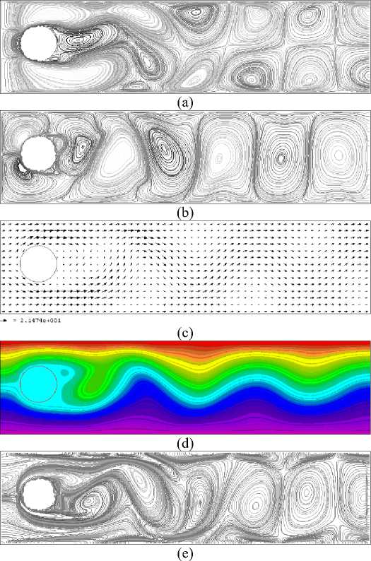
Fig. 3: Instantaneous flow around circular cylinder for Re=100, (a) axial velocity contours, (b) vertical velocity contours, (c) vector plot, (d) stream function plot, (e) vorticity contours.

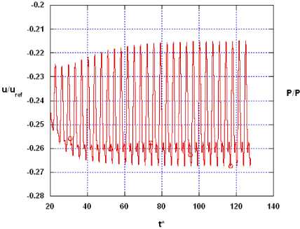
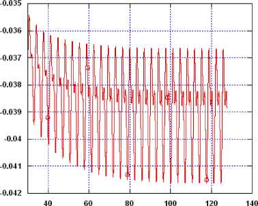
Figures (4-a, b) show the instantaneous axial velocity and pressure at x/d=2.5 for Re=100 in the downstream direction. The oscillating behavior of flow characteristics is clearly visible due to the shedding of vorticity structure behind the cylinder. Higher harmonics can also be seen in the velocity and pressure profiles revealing the well prediction of flow-acoustics interaction.

(a)

Fig. 4: Instantaneous (a) axial velocity; (b) pressure at x/D=2.5 downstream the circular cylinder, Re=100.

t

(b)

In our previous work [25] and [26], the validation of our developed numerical scheme has been carried out by performing a number of two-dimensional validation test cases concerning laminar and turbulent two-phase flow with different interfacial stresses. In such context, the accuracy of the presented developed algorithms has been estimated and proved. In general, the previous validation cases have demonstrated the viability of our numerical method and the associated algorithms in two-phase turbulent flow

• 4.    Results and Discussion

The dynamics of a circular drop usually include deformation, collision with other drops and disintegration. Turbulence can alter the outcomes of collision process[27] and [28]. The process of deformation and disintegration of a single droplet exposed either to turbulent uniform or Power-law velocity air stream is recently investigated in [29]. In the present section, different cases are selected to represent such dynamics and its related processes for colliding of two equally droplets in the so-called head-on collision process. The computational domain for such problem can be seen in figure 5.

The computational domain has 101x101 grid points in x and y directions, respectively. The uniform grid distance is given as x= y=1.0e-4 m. The droplet diameter is considered 0.001m. The time step is chosen as small as possible to ensure the stability of the computational algorithms and equals 0.8e-5s. No-slip boundary conditions are applied for all the boundaries of the computational domain.

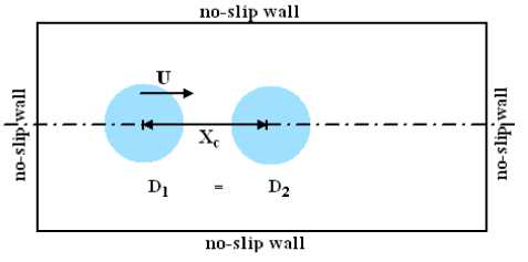
Fig. 5: Initial configurations for two colliding droplets.

Initially, two equally droplets are located head-on in stagnant gas. The moving droplet is called the "ejected" droplet, while the other is called the "target" droplet. The distance between the centres of the droplets is denoted by Xc. The dimensionless numbers control such collision process are the Weber number (We), Reynolds number (Re), and Ohnesorge number (Oh) [30]. The definition of such numbers and its values for the cases under consideration are shown in Table I.

Table I. Computational data for the different cases considered

Flow regime	Case Study	We ( ρ u2D/ σ )	Re ( ρ uD/ µ )	Oh (We0.5/Re)	X c /D
Laminar	Case I	339	133.3	0.14	1.1
	Case II	339	133.3	0.14	1.5
Turbulent	Case III	1356	266.7	0.14	1.1
	Case IV	1356	266.7	0.14	1.5

• 4.1.    Colliding of Two Equal Droplets in Laminar Regime

The considered cases I and II are performed with relatively low We and Re reflecting the dynamics of collision process in laminar flow regime. The predicted dynamics for two different values of droplet centre to centre distance Xc/D are shown in figures 6, and 7. The dimensionless numbers are kept the same for the two cases. The results show the effect of increasing the centre to centre distance on the collision outcomes and the collision dynamics as well. In all cases considered, the ejected droplet is deformed according to the bag breakup mechanism [29]. In case of Xc/D=1.1, shown in figure 6, the bag break-up mechanism is not completed due to the small distance between the two colliding droplets. As the ejected droplet has coalesced with the target droplet, the deformation process and, consequently, the break-up process are further advanced due to the initial kinetic energy of the ejected droplet. Finally, two equally droplets similar to the initial ones are formed in the transverse direction.

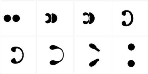
Fig. 6: Case I, collision of two equally Droplets at different time steps for We=339, Re=133.3, Xc/D=1.1, Laminar regime.

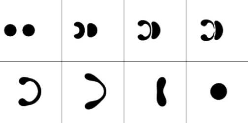
Fig. 7: Case II, collision of two equally Droplets at different time steps for We=339, Re=133.3, Xc/D=1.5, Laminar regime.

In case of Xc/D=1.5, figure 7 shows the collision dynamics for case II, where the bag break-up mechanism of the ejected droplet is partially completed. The break-up is occurred for normally for the ejected droplet. However, after the coalescence of the ejected droplet with the target droplet, a single large droplet is formed.

No break-up is observed in this case for the formed large droplet. This can be referred to the dissipation of the initial kinetic energy of the ejected droplet as a result of the viscous effects of the induced gas flow. The larger distance Xc/D enables more dissipation of the kinetic energy than the smaller distance. Figures 6 and 7 show the effectiveness of the level set algorithm in predicting merging and breaking of droplets in natural way without any numerical constraints.

• 4.2.    Colliding of Two Equal Droplets in Turbulent Regime

Dynamics of droplets in turbulent flow is one of the most important processes in reaction engineering. Although such processes are previously thoroughly investigated, however, the numerical simulation of such processes is scarce as a result of the complexity encountered. The interaction mechanisms between the turbulent structure and droplets whose dimension is much larger than the smallest dissipating eddies make the numerical prediction of such processes as the most challenge problem in computational fluid dynamics [28].

Therefore, in the present section, a numerical prediction for the collision dynamics of two equally droplet in turbulent flow regime is carried out. Both of the Weber number and the Reynolds number are increased accordingly, while the Ohnesorge number remains unchanged in comparison with the previous cases shown in figures 6, 7. The considered dimensionless numbers of the turbulent cases (Case III, and Case IV) are shown in Table I.

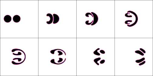
Fig. 8: Case III, collision of two equally Droplets at different time steps for We=1356, Re=266.7, Xc/D=1.1, Turbulent regime.

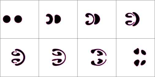
Fig. 9: Case IV, collision of two equally Droplets at different time steps for We=1356, Re=266.7, Xc/D=1.5, Turbulent regime.

Figure 8 shows the turbulent collision process for relatively small center to center distance, Xc/D=1.1. As a result of the high initial kinetic energy of the ejected droplet, the bag break-up mechanism is completed until the formation of two small droplets. The target droplet is also affected by the high kinetic energy and goes through a bag break-up process. Finally, four ligaments can be observed due to the breakup of both ejected and target droplets. The ligament might go further in secondary breakup or form permanent droplets. By increasing the distance Xc/D between the two colliding droplets, as shown in figure 9, the break-up mechanism for the ejected droplet is totally completed and the formation of ligaments followed by the formation of two small droplets is clearly visible. The target droplet is also deformed and broke-up into small droplets. The viscous dissipation of the initial kinetic energy, in case of larger Xc/D, might result in no ligament formation, however, final permanent droplets.

• 4.3.    Effect of Different Flow Regimes Considered

• 5.    Conclusion

The comparison between the flow regimes considered for the same center to center distance, (as shown in figure 6 and figure 8 or as shown in figure 7 and figure 9), show that the dynamics of the collision is performed faster in turbulent flow regime due to the relatively high initial kinetic energy and the associated high Weber number. Moreover, no coalescence of the two colliding droplets can be observed in case of turbulent flow for the same centre to centre distance considered. It can be expected that a permanent coalescence could be obtained in turbulent flow for larger values of Xc/D. Moreover, the viscous dissipation is found to be much more effective in laminar flow than that found in turbulent flow regime. This can be referred to the increase of the diffusion process and mixing enhancement in turbulent flow.

A new interfacial marker-level set method for predicting the dynamics of turbulent two-phase flows with moving interface has been developed. The governing unsteady RANS-equations are coupled with the level set method and solved in each phase separately on structured cell centred collocated grids using the control volume approach on the physical domain of the problems considered. The prediction of the well known Von-Karman vortex street problem over a fixed circular cylinder was considered as a validation test case of our developed numerical method. The numerical method has been further applied for simulating the collision process of two equally droplet in either laminar or turbulent flow regimes. The results showed the effect of centre to centre distance of the colliding droplets on the final collision outcomes, where either separated small droplets or large permanent droplets were found. The collision dynamics is performed faster in turbulent flow regime due to the relatively high initial kinetic energy. Moreover, the effect of the viscous dissipation in laminar flow regime is much more effective than that found in turbulent flow regime.

• [1]    Fuster, D., Agbaglah, G., Josserand, C., Popinet, S. and Zaleski, S., Numerical simulation of droplets, bubbles and waves: state of the art, Fluid Dyn. Res. 41:1-24, 2009.

• [2]    Lefebvre, A. H., Atomization and sprays, Hemisphere Publishing Corporation, 1989.

• [3]    Kolev N.I., Multiphase flow dynamics: Thermal and Mechanical Interaction", Springer, 2007.

• [4]    Yang V., Habiballah M., Hulka J. and Popp M., Liquid Rocket Thrust Chambers: Aspects of Modeling, Analysis, and Design", American Institute of Aeronautics and Astronautics, Inc., 2004.

• [5]    Linne M., Paciaroni M., Hall T., and Parker T., Ballistic imaging of the near field in a dense spray", Exp. Fluids., 49(4): 911-923, 2006

• [6]    Menard T., Tanguy S. and Berlemont A., Coupling level set/VOF/ghost fluid methods: Validation and application to 3D simulation of the primary break-up of a liquid jet, Int. J.Multiphase Flow, 33:510-524, 2007.

• [7]    Desjardins, O., Moureau, V. and Pitsch, H., An accurate conservative level set/ghost fluid method for simulating turbulent atomization, Journal of Computational Physics, 227: 8395–8416, 2008.

• [8]    Hinze JO., Turbulence, New York, McGraw-Hill, 1959.

• [9]    Eggers, J., Nonlinear Dynamics and Breakup of Free-Surface Flow, Rews. Modern Phys., 69(3): 865– 929, 1997.

• [10]    Crowe C. T., Troutt T. R. and Chung J. N., Numerical models for two-phase turbulent flows", Annu. Rev. Fluid Mech., 28:11-43, 1996.

• [11]    Shinjo J. and Umemura A., Simulation of liquid primary breakup: Dynamics of ligament and droplet formation", Int. J. Multiphase Flow, 36(7): 513-532, 2010.

• [12]    Rgea S., Bini M., Fairweather M. and Jones W. P., RANS modelling and LES of a single-phase, impinging plane jet, Computer and Chemical engineering, 33: 1344.1533, 2009.

• [13]    Launder, B. E., Spalding, D. B., The numerical computation of turbulent flow, Computer Methods in Applied Mechanics and Engineering, 3(2): 269-289, 1974.

• [14]    Nichols B. D. and Hirt C. W., Methods for calculating multi-dimensional, transient free surface flows past bodies, Proc. First Int. Conf. Num. Ship Hydrodynamics Gaithersburg, 20–23, 1975.

• [15]    Osher S. and Sethian J. A., Fronts propagating with curvature-dependent speed: algorithms based on Hamilton–Jacobi formulations, Journal of Computational Physics, 79: 12–49, 1988.

• [16]    Li, Z., Jaberi, F. A. and Shih, T., A hybrid Lagrangian–Eulerian particle-level set method for numerical simulations of two-fluid turbulent flows, Int. J. Num. Methods in Fluids, 56: 2271-2300, 2008.

• [17]    Scardovelli, R. and Zaleski, S., Direct numerical simulation of free-surface and interfacial flow, Annu. Rev. Fluid Mech., 31: 567–603, 1999.

• [18]    Peters N., Turbulent combustion", Cambridge University Press, Cambridge, UK, 2000.

• [19]    Balabel, A., Binninger,B., Herrmann, M., and Peters, N., Calculation of Droplet Deformation by Surface Tension Effects using the Level Set Method, Combust. Sci. Technology , 174(11-12):257–278, 2002.

• [20]    Sussman, M., Smereka, P. and Osher, S., A level set approach for computing solutions to incompressible two-phase flows, J. Comp. Physics, 114: 146-159, 1994.

• [21]    Sethian, J. A. and Smereka, P., Level Set Methods for Fluid Interfaces, Annu. Rev. Fluid. Mech., 35: 341-372, 2003.

• [22]    Brackbill, J. U., Kothe, D. B. and Zemach. A., A Continuum Method for Modeling Surface Tension, J. Comp. Physics, 100: 335-354, 1992.

• [23]    Balabel A., Numerical simulation of Gas-Liquid interface dynamics using the level set method, Dissertation, RWTH Aachen, Germany, 2002.

• [24]    Griffin O. M. and Hall M. S., Review: vortex shedding lock-inand flow control in bluff body wakes, ASME J. Fluids Eng., 113: 526-537, 1991.

• [25]    Balabel A., Numerical prediction of turbulent thermocapillary convection in superposed fluid layers with a free interface, Int. J. Heat Fluid Flow, 32:1226–1239, 2011.

• [26]    Balabel A., Numerical Modelling of Turbulence-Induced Interfacial Instability in Two-Phase Flow with moving Interface, Applied Mathematical Modelling, 36:3593-3611, 2012.

• [27]    Narsimhan, G., Model for drop coalescence in a locally isotropic turbulent flow field, J. of Colloid and Interface Science, 272:197–209, 2004.

• [28]    Ronnie, A. and Bengt, A., On the breakup of fluid particles in turbulent flow, AIChE, 52 (6):2020-2030, 2006.

• [29]    Balabel A., Numerical prediction of droplet dynamics in turbulent flow, using the level set method, International Journal of Computational Fluid Dynamics, 25(5): 239-235, 2011.

• [30]    Bayvel, L. and Orzechowski, Z., Liquid Atomization", Taylor and Francis, London, 1993.

  
  
  

  Ashraf Balabel was born in Minoufiya, Egypt, on December 12, 1965. He received the B.Sc. (the first-class, Excellent with Honors Degree), and M.Sc. degrees in Mechanical Power Engineering from Faculty of Engineering, Minoufiya University, Shebin El-Kom, Egypt, Ph.D. degree in Mechanical Engineering, from RWTH-Aachen University, Germany, in 1988, 1995, and 2002, respectively. In 1990, he became a Demonstrator at Minoufiya University, and then was an Assistant Lecturer in 1995. In 2002 was a Lecturer, in 2008 he

became an Associate Professor in the same faculty and university till now. His research interests include Thermo-Fluid Dynamics, CFD, Two-Phase flow, Turbulence Modelling, Droplet

Dynamics, Level Set Method, and Renewable Energy.