Numerical Simulation of Transient Gauss pulse Coupling through Small Apertures

Published Online August 2011 in MECS

Because of steep rising front edge, short duration time and wide spectrum, transient electromagnetic pulse (EMP) can easily couple into the internal structure of missiles or aircrafts through apertures and slots [1]. Lots of essential openings in the shell of targets, such as hot-radiating windows and data openings, provide the coupling path for transient EMP. Once the electromagnetic energy couples into the targets, the inner equipments can be disturbed, destroyed or damaged. So the work to research aperture coupling mechanism of transient EMP has important signification.

Gauss pulse is a kind of transient EMP, which can easily coupling through small apertures. Until now, researchers have studied the coupling effects of high power EMP for a number of years, and lots of

Manuscript received March 30, 2011; revised June 1, 2011; accepted July 1, 2011.

conclusions are gotten via numerical simulation [2,3]. The Finite difference in time domain (FDTD) algorithm is one of these methods which always be used to calculate the coupling course of high power EMP [4]. Kashyap and Louie have used FDTD method to analyze the interaction of HPM with complex structures [5]. They have also calculated the HPM fields scattered by a target with openings using MOM method [6]. Chevalier and S e rafin have presented a near field measurement technique to analyze the coupling effects of EMP[7]. Some researchers have studied the coupling effects on shielding cables with FDTD algorithm. Casey and Vance studied the coupling mechanism of EMP through cable shields in 1978 [8]. Mccormick estimated induced-voltage peak magnitude and energy level under EMP excitation of low-loss aircraft cable [9].

Apertures with centimeters are studied by researchers [10, 11], while apertures with millimeters are studied less. One reason is that the divided number of space grids will be very great and make great waste of calculation time , if the small aperture is very small compared with the whole calculation space. So sub-gridding technique can be used to solve this problem. It not only can simulate these small apertures accurately, but also can save the computer memory resource.

Coupling course of Gauss pulse through small apertures is modeled and simulated using sub-gridding FDTD algorithm in this paper. The affect on coupling effects illuminated by varied incident angles and varied pulse width is studied. Some coupling rules about electric field strength and power density are gotten, including resonance effect in the cavity and coupling increase effect of rectangle aperture. These results can help us to understand the aperture coupling mechanism of transient Gauss pulse.

• II.    FDTD Algorithm and Aperature Coupling

• A. FDTD Algorithm

If the equipment shells with apertures in it are illuminated by transient Gauss pulse, we know that coupling phenomenon through apertures and reflection phenomenon by shells will happen. The two phenomena both can be described with Maxwell’s equations in electromagnetic theory. So we start with the Maxwell’s equations.

∇×H=ε∂E+σE ∂t

∇× E =- µ ^∂ H - σ _m H

∂ t

Where E is the electric field vector,

H

is the

magnetic field vector, ε is the media electric constant, σ is the electric conductivity, µ is the magnetic

conductivity coefficient, σ _m is the magnetic conductivity.

In Descartes coordinate system, the Operator “ ∇ ” can be written into

v ∂ v ∂ v ∂

∇= i + j + k

∂ x   ∂ y ∂ z

.

For (1) it gives

i

∇× H =

∂ ∂ x

H x

^j ∂ ∂ y H y

k

∂ ∂ z

.

H z

Then (1) can be produced into three scalar equations, which is as follow.

dH	∂ H	∂ E
z	- y	= ε x	+ σ E	(5.a)
∂ y	∂ z	∂ t	x
ан	∂ H	∂ E		(5.b)
x	- z	= ε y	+ σ E
∂ z	∂ x	∂ t	y
∂ H	∂ H	дЕ
y	- x	= ε z	+ σ E	(5.c)
∂ x	∂ y	∂ t	z

We rewrite each scalar equation in finite difference form. Taking (5.a) for example, after transformed into difference form in time domain, it can be written into

H z ^{n + 12}( i + ¹2 , j + ¹2 , k ) - H z ^{n + 12}( i + ¹2 , j - ¹2 , k )

Δ y

_- H y ^{n + 12}( i + ¹2 , j , k + ¹2 ) - H y ^{n + 12}( i + ¹2 , j , k - ¹2 )

^{Δ z}                       (6)

_{= ε ( i +} 1 _{2, j , k )} E x ^{n + 1} ( i + 12 , j , k ) - E x ⁿ ( i + 12 , j , k )

Δ t

E^{n + 1} ( i + ¹2 , j , k ) + Eⁿ ( i + ¹2 , j , k ) + σ ( i + ¹ ₂, j , k ) ^x 2 ^x

.

Where Δ y is grid length in direction Y, Δ z is the grid length in direction Z, Δ t is the length of time step, n is the ordinal number of time step, and ( i , j , k ) is the ordinal number of space step. Equation (6) is actually provides us the finite difference approximations. If E_xⁿ , H_z^{n + 12} and H_y^{n + 12} are known, we can calculate E_x^{n + 1} by this recursion equation.

Using this method, we can get other two recursion equations deduced from (5.b) and (5.c). Equation (2) can be deduced using this method too. Then we actually get six recursion equations, which is used to calculate the value of E_x , E_y , E_z , H_x , H_y and H_z respectively.

There are two main problems for numerical simulation of aperture coupling. One is how to simulate the coupling course in time domain, and the other is how to model the

small aperture accurately.

Because the Maxwell’s equations are linear equations, the electromagnetic field can be split into two fields, namely incident field and scatter field. For numerical simulation of aperture coupling effect, we concern total field problem. The total field gives

Where E ^total

E

total

= Einc

+ E

scatter

H total ₌ H inc ₊ H scatter and H ^total are the total

(8) field of

electromagnetic wave, E ^inc and H ^inc are the incident field, E ^scatter and H ^scatter are the scatter field. If the electromagnetic field is split into incident field and scatter field, because incident field can be solved analytically in the whole calculation space, then scatter field is the only left one needs to be numerical analyzed.

FDTD calculation area of electromagnetic coupling problem is shown in Fig. 1. The whole calculation area can be divided into total field area and scatter field area. The two areas are connected by the connect border, and the incident wave source is loaded on the connect border in calculation.

B. Calculation Space Model

The calculation space model is shown in Fig. 2.We use a cubic shield cavity, which is marked by solid line, to simulate the equipment shell, in which there are one or several apertures with variable shapes. Length of each side is 200 mm, and depth of cavity shell is 2mm.

absorbing border condition

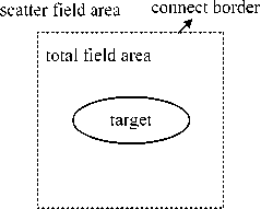
Figure 1. FDTD area partition of electromagnetic coupling problem

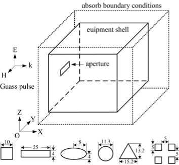
Figure 2. Calculation space model of aperture coupling

Six kinds of apertures, which have same area but different shapes, are selected to research in this paper. They are square, rectangle, ellipse, circle, triangle and square array aperture respectively, and the area of each aperture is 1 cm2. Detailed size of these apertures is also shown in Fig. 2. The outer layer marked by dotted line is the absorbing border. The incidence of Gauss pulse is in direction k. Base on this calculation space model, coupling effect of transient Gauss pulse through small aperture is studied at varied pulse characteristics, including pulse width, incident angle, etc.

• C.    Calculation Steps of FDTD Method

Electromagnetic simulation of aperture coupling problem using the FDTD method can be divides into 8 steps. The calculation flow is as follows:

Step1 : Difference of Maxwell equations in time domain. The FDTD finite difference approximation equations art gotten.

Step2 : Calculation of time step length and space step length of Yee grid. The basic cell dimension should be calculated in three-dimensional space.

Step3 : Selection of calculation space. Firstly, the whole targets should be loaded in the calculation space. At the same time, connect border setting should be considered.

Step4 : Setting of absorbing border condition along the outer surface of calculation space.

Step5 : Loading of the incident pulse source.

Step6 : Evaluation the total number of time steps and total store capacity of computer. In this step, the coupled pulse should be reach steady state.

• D.    Some Restriction Conditions

To ensure the convergence of numerical simulation, some restriction conditions about space grid and time step should be considered. Considering the stability of FDTD algorithm, length of space grid should satisfy the following equation [4].

А< X 12 (9)

Where А is length of the space grid, and X is length of the incident pulse. While selecting the length of time step, it should satisfy the following equation [4].

А t <  T /12 (10)

Where А t is length of the time step, and T is period of the incident pulse. Cubic Yee cells are often used when calculating the space grid, namely А = A x = А у = A z .

• III.    Sub-gridding Approach and Application

• A. Sub-gridding Divided Method

While dividing the calculation space, even grids are usually used in numerical simulation. It is very convenient for calculating the total space grids and time steps using even grid dividing technique, but even grids have its disadvantage. If the small aperture is very small compared with the whole calculation space, the divided number of space grid will be very great. This will make great waste of calculation time and computer memory resource. One approach to solve this problem is using the sub-gridding technique to divide calculation space.

There are several kinds of sub-gridding divided approaches. The shaded grid divided approach [12] is used and discussed in this paper. The detailed steps are as follows:

We suppose the total number of three-dimensional sub-gridding calculation space is n_x x n_y x n_z , where n_x , n_y and n_z are the number of grids in direction X, Y and Z, respectively. Then one arbitrary vertex in calculation space can be noted as ( x i , y j , z k ) , where 1 <  i <  n_x , 1 <  j <  n_y , 1 <  k <  n_z . Taking conformation of sub-gridding in direction X for example, the divided approach is shown in Fig. 3.

We suppose length of the ith grid step on direction X is

Ax,-= Xi- xi4,

Where i = 1, l , nx . Then the distance between two centers of border (shown in Fig. 3) can be defined as dx, = X+1/2 — Xi-1/2 = (Ax i+1 + Axi)/2.

Where i = 1, l , n_x . For the sub-grids, length of grid increases step by step as the power of prolate gene increases. Length of the ith grid is

Ахi=Ax1 qx -1

.

Where Ах1 = x1 - x0, qx is the prolate gene, the value of which is 1 < qx < 1.3 . Then coordinate of the ith grid in direction X is xi = xi-1 + Axi = xi_1 + Ax 1 qx 1

The distance between two centers of border calculated using the prolate gene.

d_x = 1/2 A x q i - 1 (1 + q ,)

x _i    1 xx

(14) can be

We can calculate length of space grid in direction Y and Z with the same approach. After coordinates of subgrids are gotten, we should deduce the FDTD recursion equation for sub-grids.

Firstly, we note the electric field and magnetic field of sub-grids in direction X is

E n ( i +1, j , k ) = E x ( x _u 2 , у ^ ,Z k , n А t ),     (16)

H x ^{+ 2}( i , j + 1 k + 1)

= H x ⁽ x , У + 2 , ^zk + 1 ^,( n ⁺В^А t )

.

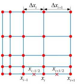
Figure 3. Sketch of sub-gridding divided method

Because transmit media has the characteristic of isotropy, FDTD difference equations for sub-grids in time domain give

E " ^{+ 1} ( i +2, j , k ) = E X ( i +1, j , k ) + - x

7

• { -7 [ H z ^{+ 2} ( i + b j + 2 , k ) - H z ^{+ 2}( i + b j - b k )] (18)

_dyj     22      22

- -¹-[ H " ^{+ 2} ( i +1, j , k + j) - H " ^{+ 2}( i + 2 , j , k - i)]}

z k	A z i = A z i _ 1 + A z x r ' ( b + 1)	(24)
H X + 2( i , j +1 k + 2 ) = H X - 2( i , j + 2, k + 2)	A z = A z b + 1 - A zb	(25)
+ ^ t {-7 [ E X ( i , j + 2 , k + 1) - E " ( i , j + 2 , k )] (19) M dz k	Az ь = A, b        fine b + trtrans	(26)
1	SUM = ^ A z i i = b + 1	(27)
-—[ E X ( i , j + 1, k + 1 ) - E X ( i , j , k + 1 )]}

y j

The electric field and magnetic field in direction Y and direction Z have the similar form. FDTD difference equations for sub-grids in direction Y give

E " ^{+ 1} ( i , j +1 k ) = E " ( i , j +1 k )

A t , 1

+7{T zk

[ H " ^{+ 2} ( i , j ₊ 2 , k ₊ -2 ) - H " ^{+ 2} ( i , j ₊ 1 , k - 1)] (20) Absorbing boundary conditions are necessary to keep outgoing electromagnetic field from being reflected back

• -    -7 [ H z ^{+ 2}( i +b j +1, k ) - H z ^{+ 2} ( i - b j +b k )]}

d_xi     22      22

H " + ² ( i + 2 , j , k + 2) = H " - ² ( i +1 j , k + 2)

• + - {"Г [ E X ( i + 1, j , k + D - E " ( i , j , k + 2)] ( M d_x,

• -    -¹- [ E " ( i + 2, j , k + 1) - E " ( i + 2, j , k )]}

d_zk  22

FDTD difference equations for sub-grids in direction Z give

E z ^{+ 1} ( i + 2 , j , k + 2) = E z ( i + 2 , j , k + 2)

A t , 1

+7{X xi

[ H" ⁺ 2 ( i + 2 , j , k + 1) - H" ⁺ 2 ( i - 2 , j , k + !)] (22) condition (ABC) is set in the edge area of calculation ^yy      space.

• -    -7 [ H X ^{+ 2} ( i , j + 2 , k + 2) - H X ^{+ 2}( i , j - 1 k + 2)]} _dyj     22      22

H z ^{+ 2} ( i +1 j + 2 , k ) = H z - ² ( i + 2, j + 2 , k )

• +    ^ t {"^ [ E X ( i + 7, j + 1, k ) - E X ( i + b j , k )] (23) M dy,

• -    -7 [ E X ( i + 1, j + 2, k ) - E " ( i , j + -2, k )]} d 22

x _i

Thus, we get sub-gridding FDTD difference equations. If we know the in value , transmitting and coupling course of transient Gauss pulse can be calculated and simulated in time domain using (18) - (23).

• B.    Application for modeling small apertures

Because of very short width of the aperture, sub-gridding technique are used to simulate the small aperture. Taking rectangle aperture for example, Fig.4 is the sketch of space grid partition of the rectangle aperture, in which the non-uniform grids in z direction can be seen. The fine grids are used to simulate the width of the slot, and the coarse grids are used to simulate the main area. The length of fine and coarse grid is A fine and A coarse , respectively. There is a transitional area between fine grids and coarse grids. Supposing the grid number of the transitional area is ntrans and the number varies from b +1 to b + "trans, the grid length in transitional area can be described as

Where A z i is the length of the i th grid in z direction. r is an increasing gene, and it satisfies 1 <  r <  1.5 . i satisfies b + 1 <  i <  b + n trans . SUM is the sum of grid length in the transitional area. SUM should be selected as an integer to improve the exactness of calculation.

into the problem space. A seven-point PML absorbing boundary conditions [4] are used in this paper.

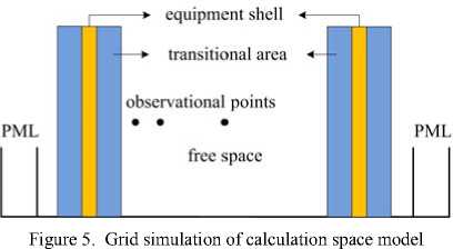
Aperture size is very small compared to the whole cubic cavity, so sub-gridding approach is used to simulate these small apertures. To simulate these small apertures accurately, cavity shell and apertures in it are modeled with fine grids. Fig. 5 shows sub-grids setting approach of the cavity shell. In this figure, yellow area represents equipment shell, which is simulated with 4 fine grids. Blue area represents transitional area, which is divided with sub-grids. It is free space, which is modeled with coarse grids, in the cavity. Length of each fine grid is 0.5mm, and length of each coarse grid is 2mm. Finally, the perfect matched layer (PML) absorbing border

• C.    Gauss Pulse Loading Method

Function of Gauss pulse in time domain gives

E , (t ) = E о x exp[ - ^{4П ( -} - ^{- o )} ]        (28)

т

Where E ₀, 1 ₀ and т are constants. Gauss pulse width is decided by т , and peak value of pulse appear in time t ₀ . Function of Gauss pulse in frequency domain can be gotten through Fourier transformation of (28). It is as follow:

E ( f ) = E о x T 2 x exp( - j 2 n ft о - n f ² т ² / 4) (29)

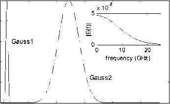
We select two kinds of Gauss pulse with same magnitude but different pulse width to research, marked as Gauss1 and Gauss2, respectively. Their parameter values are listed in Tab. 1.

Fig. 6 shows waveforms in time domain of these two pulses calculated via (28). From the figure, we can see that common characteristics of two waveforms are steep rising front edge, short duration time and high electric field magnitude. For example, duration time of pulse Gauss1 is only 128ps, and pulse width is about 87 ps, while pulse width of Gauss2 is about 1.5 ns, which is 9 times larger than Gauss1 pulse. The spectrum is also shown in the top right corner of Fig. 6. We can see that spectrum of Gauss pulse is very wide, which range from several hundred MHz to several GHz. These characteristics make Gauss pulse easy to coupling into the inner of equipments via apertures.

How to load wave source in the calculation space may be a problem which we should solve before simulation. Firstly, we suppose that equipment shell is in the far field area of wave source, then we can load incident pulse in calculation space with plane wave. We can use the method of loading incident pulse in the corresponding Yee grid gradually, according to the time step. Taking plane XOY as an example, there are M by N grids in this plane, which is shown in Fig. 7. The loading plane is in the shadow area. Electric field value of the second grid plane YOZ gives

E z ⁿ (2, j , k ) ← E z ⁿ (2, j , k ) + F ( n Δ t ) (30)

Where E_zⁿ (2, j , k ) is electric field in direction z at grid (2, j, k), and n represents the time step. As time step increases, according to recursion formula, incident pulse is loaded in calculation space gradually, and transmits in direction X. Thus, simulation of the incident plane wave is achieved. Only a single pulse is studied in this paper.

TABLE I. P arameter V alues of G auss P ulse

Pulse type	Parameter value
	E 0 (V/m)	t 0 (s)	τ (s)
Gauss1	1000	1.22×10-10	9.4×10-11
Gauss2	1000	1.22×10-9	9.4×10-10

A—coarse grid area B—transitional area

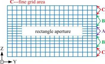
Figure 4. Sub-gridding simulation of rectangle aperture

• D.    Calculation Flow for Aperture Coupling

Calculation flow for the small aperture coupling problem is shown in Fig. 8. Firstly, the number of time step is initialized to one. Secondly, the electric field is interpolated in spatial space and updated with the FDTD recursion equation. Then the same work is done to the magnetic field. After this, we need to judge whether n is equal with n R , which is the total number of time step. If n is less than n R , n is replaced by n+1, and the calculation course goes on. If n is equal with n R , the simulation work is over.

0        0.5        1        1.5        2        2.5        3

time (ns)

Figure 6. Waveform of two kinds of incident Gauss pulse

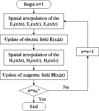
Figure 8. Calculation flow for small aperture coupling

A t =2-7ps and n R =7500 are selected in this paper calculated by (10), so the coupling time through apertures for Gauss pulse is about 20 ns. A little long time will be needed for running of this program.

• E.    Coupling Coefficient Definition

To calculate coupling effect through small apertures in the inner of equipment shell, we define “coupling coefficient” to compare the coupling degree, namely the ratio of coupled power to incident pulse power at this point, marked with n - The expression is n = 10lg(Pcoup I P„c ) = 20lg(Ecoup I Enc ) - (31)

Where P_inc and E_inc are power and electric field strength of incident pulse at the front cross section of aperture, P_coup and E_coup are power and electric field strength of coupled pulse at some cross section in the cavity, respectively. The expression of P_inc and P_coup is

P c = J _S ( E c ■ H nc ) dS ,          (32)

P cou = J S ( E coup ■ H coup ) dS -          (33)

Where H nc represents magnetic field magnitude of incident wave at the front cross section of aperture, Hcoup represents coupled magnetic field magnitude at the back cross section of aperture, and S represents the cross section proportion of aperture.

Power density at some point in the cavity can be calculated with vector S . Its expression in Descartes coordinate frame gives

v

S = E X H = ( E y H z - E z H y ) i

vv

+ ( E_ZH_X - E_XH_Z ) j + ( E_XH_Z - E_ZH_X ) k zx xz    xz zx

The coupling resonance frequency in cavity can be estimated with the following equation [83].

f = 0.5 c tJ ( ml a ) ² + ( n/b ) ² + ( p/h ) ²      (35)

Where a, b and h is the length, width and height of this cubic cavity, respectively. m, n and p is the module of resonance wave. c is the wave velocity.

For the cubic cavity in this paper, the resonance frequency of wave TE101 is 1.06 GHz, calculated by (35).

• IV. Numerical Results and Discussion

• A.    Coupl ng Effects of Square Aperture

Taking plane ZX for example, we study the coupling course in the center of cavity. Time step number is marked as n. Fig. 9 is electric field contour map of plane ZX in the center of cavity at varied time steps. Abscissa is the x-axis coordinate, and ordinate is the z-axis coordinate. Coupling course can be observed clearly from this figure. Where (1) shows Gauss pulse is coupling through aperture; (2) shows main pulse is going to reach the back wall of cavity, and then reflects; (3) shows reflected main pulse transmits to the neighborhood of aperture, and radiates energy through the small aperture, which likes an antenna at the moment; (4) shows electromagnetic energy scatters in the cavity, after surge and leaking times without number.

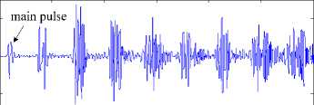
Fig. 10 shows coupled electric field waveform at several points in the axial line of square aperture. We select four points to study, which are inner center of aperture, place 1cm to aperture, place 3cm to aperture and center of cavity, respectively. The first pulse of each waveform is the couple main pulse, and other pulse after main pulse is the reflected pulse by back shell of cavity. According to calculation results, we know that the time for pulse to transmit from the center to back wall and return to the center of cavity is 1.33 ns, which is the surge period of coupled pulse actually. Obviously, interior resonance phenomenon happens between Gauss pulse and cavity. But the coupled electromagnetic energy radiates through apertures at the same time, which makes the coupled electric field magnitude attenuates gradually. From (c) and (d), we can see that the second pulse and the third pulse are larger than main pulse. This enhancement phenomenon after main reflected pulse can be explained mainly by the reflected effects of cavity side shell.

Coupled electric field through square aperture in the center of cavity in frequency domain is shown in Fig. 11. To observe the coupling rule conveniently, Smoothing work is done to the original data. The resonance point in the cavity of TE101 wave is 1.06 GHz calculated by (10), which is same as the first resonance point in the figure. From the figure, we also can see that coupled electric field magnitude in the high frequency domain from 8 GHz to 15 GHz is bigger than the one in low frequency domain. This phenomenon can be called high-frequencypass coupling characteristic.

Power density magnitude in the axial line at different time steps is shown in Fig. 12. Because coupled electromagnetic pulse leaks through small aperture, electromagnetic energy attenuates as the time step increases. Power density is 96.5 W/m2 at the 131st time step, and gradually decreases to 19.9 W/m2 at the 6991st time step.

• B.    Rectangle Aperture

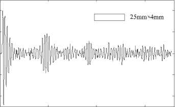
To compare coupling effects of rectangle apertures with different ratio of length to width, two kinds of rectangle apertures are selected to study. Length and width of aperture Rectangle1 is 25mm and 4mm, while length and width of Rectangle2 is 50mm and 2mm.

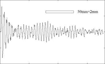
Coupled waveforms for these two kinds of rectangle apertures in the inner center of apertures are shown in Fig. 13 and Fig. 14. We can see clear increase effect occurs around rectangle aperture from these two figures. The biggest coupled electric field strength through aperture Rectangle1 and Rectangle2 is about 2.4 kV/m and 3.3 kV/m, which is 2.4 times and 3.2 times of the incident pulse magnitude, respectively. We called this phenomenon “coupling increase effect”, which means coupled electromagnetic wave increases and bigger than the incident pulse. The reason may be that lots of electric charges are accumulated around the aperture and radiate quite high electric field in very short time.

Fig. 15 shows coupling coefficient of rectangle apertures with different ratios of length to width, where d represents the distance of the point to aperture. These two rectangle apertures have same area. From the figure, we can get this conclusion clearly that coupling coefficient is greater, if the ratio of length to width is bigger.

• C.    Apertures with Different Shapes

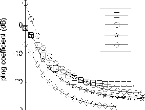
To study the affect on coupling effects of different apertures, six kinds of apertures are studied. Fig. 16 shows coupling coefficient in the axial line for apertures with different shapes. From the figure we know that: @ Coupled energy exists only around the aperture. As the observation point moves to the center of cavity, coupled energy decreases rapidly. @ Change rules of coupled electromagnetic wave of square, rectangle, ellipse and circle aperture are consistent. Coupling coefficient of triangle and square array aperture, less than -40dB, is obviously less than other apertures.

• D.    Coupling Effects with Different Pulse Duration

To compare coupling effects of Gauss pulse with different duration time, we simulate the coupling course of square aperture illuminated by pulse Gauss1 and Gauss2 respectively. Coupling waveforms illuminated by pulse Gauss1 and Gauss2 are shown in Fig. 17 and Fig. 18 respectively. The place 3cm to aperture is selected both for the two figures.

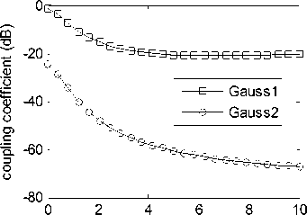
From two figures, we can see that coupled waveform illuminated by Gauss1 surge acutely, while coupled waveform illuminated by Gauss2 almost doesn’t surge. Taking the biggest coupled electric field magnitude for example, it is about 300V/m and 2V/m respectively, illuminated by Gauss1 and Gauss2. The same results can be got at other observation points. So we can conclude that it is much more easily for short Gauss pulse to couple through small aperture, than the long Gauss pulse. Fig. 19 shows the coupling coefficient in axial line illuminated by pulse Gauss1 and Gauss2.

• E.    Different Incident Angles

Oblique incidence situation of Gauss pulse is simulated with the same approach, and the only difference is incident wave loading. Firstly, we define θ as incident angle, which is the angle of incident direction and plane YZ. Coupling coefficient curve of square aperture at different incident angles is shown in Fig. 20. From the figure, we know that coupling rules at oblique incidence are similar to the one at normal incidence. We also can see that the coupling effect weakens as the incident angle decreases.

time (ns)

(b) The place 1cm to aperture

0        2        4        6        8        10       12

-200

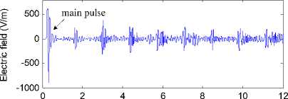
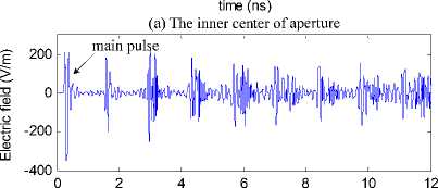
time (ns)

(c) The place 3cm to aperture

-200

• main pulse Jp^.lU>] p ^|

*H^Hkw

0        2        4        6        8        10       12

time (ns)

(d) The center of cavity

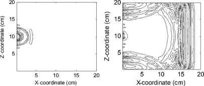
(2) n=291

(1) n=l31

E

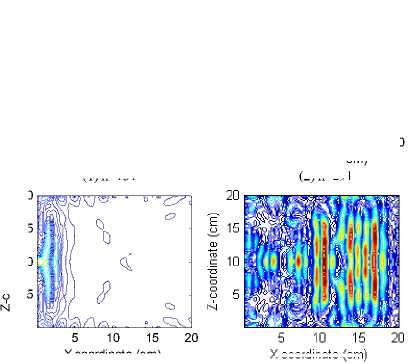
X-co ord in ate (cm)

Figure 9. Electric field contour map at ZX plane

X-coordinate (cm) (3)n=6H

(4)n=6991

Figure 10. Waveform of electric field at different position of axial line

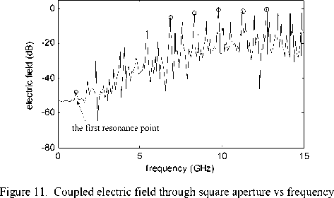
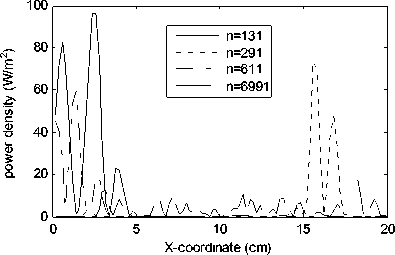
Figure 12. Magnitude of power density in the axial line

-10

square rectangle ellipse circle

-20

-30

пп пп пп нннд: ееехэее

distance to aperture (cm)

(a) Square, rectangle, ellipse and circle

Е" 1000 0 -1000 -2000

0             5            10            15

time (ns)

Figure 13. Coupling electric field in inner center of aperture Rectangle1

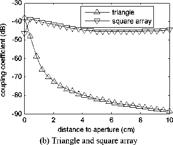
Figure 16 Coupling coefficient of apertures with different shapes

Е

-2000

0             5            10            15

time (ns)

Figure 14. Coupling electric field in inner center of aperture Rectangle2

-4000

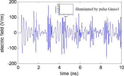
Figure 17. Coupling waveform illuminated by pulse Gauss1

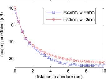
Figure 15. Coupling coefficient of rectangle apertures

Е

о

о о

-2

-4

-6

-8 0

400 I /у| illuminated by pulse Gauss2 time (ns)

ГхГ^Г-АгаЛ/Л?

46 time (ns)

Figure 18. Coupling waveform illuminated by pulse Gauss2

distance to aperture (cm)

Figure 19. Coupling coefficient at different pulse width

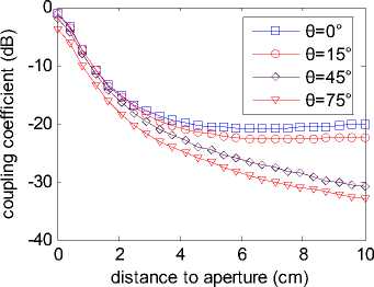
Figure 20. Coupling coefficient under oblique incidence

• [1]    Michel Camp, Heyno Garbe and Daniel Nitsch. “UWB and EMP Susceptibility of Modern Electronics”, Proceeding of IEEE Int. Symp. Electromagn. Compat., Montreal, Canada, Vol.2., pp.1015-1020, 2001.

• [2]    Liu Qiang, Zhu Zhan-ping and Qian Bao-liang, “Influence of inner slot position on the coupling of microwave into nested cavities,” High Power Laser and Particle Beams. Mianyang, vol. 19, pp. 919-922, December 2007. (in chinese)

• [3]    Fu Ji-wei, Hou Chao-zhen and Dou Li-hua, “Numerical analysis on hole coupling effects of an oblique incidence of electromagnetic pulse,” High Power Laser and Particle Beams. Mianyang, vol. 15, pp. 249-252, June 2003. (in chinese)

• [4]    Dennis M. Sullivan, Electromagnetic simulation using the FDTD method, 1st ed., New York: IEEE press, 2000, pp.79-89.

• [5]    S. Kashyap and A. Louie, “Analysis of interaction of HPM with complex structures,” Proceeding of Sensor and Propagation panel symp. on “High Power Microwaves (HPM)”, Canada, pp. 9(1)-9(9), May 1994.

• [6]    S. Kashyap, M. Burton, and A. Louie, “Calculation and measurement of HPM fields scattered by a target with openings,” Proceeding of Sensor and Propagation panel symp. on “High Power Microwaves (HPM)”, Canada, pp. 15(1)-15(6), May 1994.

• [7]    B. Chevalier and D. Sérafin, “Coupling analysis by a rapid near field measurement technique,” Proceeding of Sensor and Propagation panel symp. on “High Power Microwaves (HPM)”, Canada, pp. 16(1)-16(6), May 1994.

• [8]    F. Casey and F. Vance, “EMP coupling through cable shields,” IEEE transactions on electromagnetic compatibility, vol. 20, pp. 100-106, February 1978.

• [9]    S. Mccormick, “The estimation of induced-voltage peak magnitude and energy level under LTA/EMP excitation of low-loss aircraft cablin,” IEEE transactions on electromagnetic compatibility, vol. 21, pp. 136-146, May 1979.

• [10]    Chen Xiu-qiao,Zhang Jian-hua,Hu Yi-hua.Analysis on resonant characteristic of electromagnetic pulse coupling into narrow slot and cavity with slot. High Power Laser and Particle Beams, 2003,15(5): 481-484. (in chinese)

• [11]    Wang Jian-guo, Liu Guo-zhi, Zhou Jin-shan. Investigations on function for linear coupling of microwaves into slots. High Power Laser and Particle Beams, 2003,15(11): 10931099. (in chinese)

• [12]    Zhou Bi-hua, Chen Bin and Shi Li-hua, EMP and EMP protection, 2^nd ed., Beijing: National defence industry press, 2004, pp.121-128.

  
  
  

  Jinshi Xiao was born in Hebei Province, China. He received the doctor degree in electronic engineering from Naval University of Engineering, Wuhan, China, in 2010.

influence.

Xiongwei Ren was born in Hubei Province, China. He received the Electronic Engineering degree from Huazhong University of Science and Technology, Wuhan, China, in 2003.

He was an Associate Professor in 2004.

He has published over 20 refereed journal and conference papers in the areas of system modeling and simulation. His representative published articles list as follows: A novel model of the cross-layer architecture for wireless Ad hoc networks (China: International Conference on Wireless Communication technology, 2010) His current research interests are modeling and simulation, wireless sensor network, system theory and method.

Jiang Zhao is born in Langfang, Hebei Province, 1979. He received the Master of Engineering in system engineering from Navy Academy of Armament, Beijing, China on April 2008. His research interests include system modeling, information fusion, computational electromagnetic and electromagnetic theory.