Numerical Study of Non-premixed MILD Combustion in DJHC Burner Using Eddy Dissipation Concept and Steady Diffusion Flamelet Approach

Published Online June 2021 in MECS

Moderate and Intense Low-Oxygen Dilution (MILD) combustion is one of the most capable new techniques to increase thermal efficiency and reduce pollutant emission in the jet industry [1]. This technique is also called Flameless Oxidation (FLOX) or Highly Preheated Air Oxidation (HPCAO) or here, which is known as MILD combustion. Here, the inlet temperature of the reactants is kept relatively higher than the autoignition temperature of the mixture, and simultaneously the increase of maximum temperature is attained during combustion generally keeps lower than the temperature of auto-ignition [1]. This condition is being achieved due to the recirculation of the product gases into the arriving fresh air efficiently. The gas circulation depends on two factors: the rise of reactant temperature (heat recovery)

and a reduction in oxygen concentration, i.e., dilution. The flame temperature is relatively lower than the usual temperature ranges from 1100 K to 1500 K as dilution reacts with pre-cooled product gases.

There are many developing techniques for reducing pollutants and emissions of NOx, SO x, and CO, which results in a reduction in thermal efficiency and productivity.in combustion. MILD combustion also known as flameless combustion as during optimization conditions, there is no visibility and flame audibility at oxidation. For MILD combustion, there is still a need for valuable knowledge of flame structure, which is required to explore yet. Its principle technique lies in the exhaust gas concept and heat recirculation. The heat released from exhaust gases used for raising oxidant stream temperature and the exhaust gases used to dilute the oxidant steam on the reduction of the oxygen concentration leads to maintain a low temperature in the combustion experienced zone. MILD combustion has been experimented at Lab-scale furnaces as well as on a semi-industrial furnaces scale Plessing et. al., Danon et. al. and Orsino et al. studied a burner at the semi-industrial level through three various models of turbulent-chemistry interactions (Eddy Break up, Eddy Disspitation Concept, and PDF) presume model with the mechanism of chemistry equilibrium [2,3,4]. Mancini et al . had observed the prediction of entrainment through jets being a crucial aspect of the practical modeling approach of MILD combustion [5]. Kim et al. found global reaction mechanism effects on modeling MILD combustion of natural gas [6]. The Delft flame was implemented in a two-dimensional model using the EDC approach by De et al. [7]. It had modelled in the framework of the RANS turbulent model with methane reduced mechanism for specific Reynolds numbers. However, in this study, moderately high methane concentration fuel is accounted for to examine the behaviour of the jet with the same Reynolds number. For DJHC-I with a Reynolds number of 8800, it is observed by Kulkarni and Polifke that the second mixture fraction is lower than the other two cases [8]. Katsuki and Hasegawa focused on heat recirculating combustion effects under co-flow heated air (range of 1200 k to 1500 k). They stated that the continuous auto ignition for this highly preheated air combustion is sustainable [9]. However, in such high-temperature conditions, MILD combustion continues as variable techniques to improve fuel saving and low emissions. They also stated that when the combustion air intensively mixed with injecting fuel high momentum in the combustion chamber, it lowers the temperature of the flames and creates reactions. The system was also achieving the low NO_x and other emissions. Hence, the technology was considered as beneficial in terms of emission reduction and fuel efficiency. However, a better understanding is required regarding the change in flame structure at low oxygen level and turbulent effect shift in structure.

Plessing et al. examined a threefold drop in total emission of NO x in MILD combustion relating to standard flames where OH (Hydroxide) is homogeneously distributed on the flame burn-side [2] and reported the substantial influence on the flame structure during the interaction of turbulence and chemistry. It is observed to attain MILD combustion in the environment of the chamber, and the high-velocity shear motion inlet air is significantly needed. De Joannon et al . examined zero-dimensional oxidation analysis of methane diluted where they used Chemkin package PSR code [10]. Besides, they discovered the flameless oxidation schematization as a two-stage process where one of the methods creates rich diluted conditions. This approach had the limitation of the oxidation process of practical flameless.

The reaction zone creates a hot medium with a uniform temperature at different oxygen levels depending on the momentum of the jet and the co-flow. According to Dally et al. , laminar flow and an extreme drop in NO_x emission from the turbulent non-premixed flames reaction zone. It is stabilized on a bluff body with an increase in the recirculation rate of hot products [11]. However, few studies on the numerical investigation of turbulent non-premixed combustion in a Delft Co-flow Burner is reported. Hence, this study concentrates on the use of turbulent-chemistry interactions models of EDC and Steady Diffusion Flamelet, which is adopted in the PDF approach for numerical investigation of non-premixed MILD combustion in DJHC burner using reduced chemical kinetic schemes with 22 species (DRM 22) and GRI Mech 3.0, respectively.

2.    Experimental Setup

• A.    The Burner Design

The Delft jet-in-hot co-flow (DJHC) burner built based on the Adelaide jet-in-hot co-flow burner. Here, a fuel injets in the co-flow region of subsequently low concentration of oxygen and adequately high temperature for attaining a mixture temperature above auto-ignition after mixing. The design of the DJHC burner is sketched in Fig.1. The primary burner includes a main primary fuel jet of 4.5 mm diameter (inner), and the secondary burner produces co-flow with 82.8mm diameter. It consists of premixed and non-premixed combustion. It also includes a premixed flames ring, having additional air injectors at both sides of the ring. The partial premixed can be found for giving stability to combustion. The cooling of the central pipe is done by continuous airflow through air ducts of concentric cooling, which helps to prevent excessive heating of the main fuel jet.

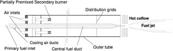
Fig.1. A schematic diagram of DJHC burner[7]

The independent oxygen (O 2 ) content-controlled co-flow temperature mimics the conditions like a real boiler where fuel gas enters aerodynamically into the near burner zone after the loss of heat from surroundings. To achieve this goal, N 2 was added with oxygen in this experiment. The temperature has been controlled with the influence of radiation and convection of heat loss from the pipe of the burner. The burner indicates that the outer wall radiates extremely at the higher distribution grid, and another grid distribution function is the mixing of the product flow circumferentially and radially in direction. The experimental evidence proves the co-flow is perfectly axis-symmetric.

• B.    Experimental and Model Database

There are series of DJHC burner experiments have been developed in different studies for various co-flow oxygen level and different Reynolds number fuel jet. Dutch natural gas, i.e., pure methane, has been considered in this study and the model study is reported depending on two different types of co-flow, as tabulated on the table. The co-flows which were used in this paper are containing Y O2 of 7.6 %.

All the measurements of the experiment and simulation have been taken along the radial profile at different location of axial, x = 3 mm, 15 mm, 30 mm, 60 mm, 90 mm, and 120 mm from the exit of the jet. The velocity of Favre average, _u and the Reynolds stress _uu are obtained using Laser Doppler Anemometry (LDA) from several instantaneous velocity measurements. The mean temperature and variance of temperature were obtained from multiple instantaneous temperature measurements through Coherent Anti-stokes Raman Spectroscopy. The oxygen concentration radial profile in the hot co-flow can be measured by using a measuring probe.

• C.    Test Cases

  The test case in this paper was carried out through the Delta Jet in Hot Co-flow (DJHC) by Oldenhof et al. [12]. Here, the fuel jet enters into a hot air co-flow with low profile oxygen. This high temperature creates an ignition of the injected fuel. The benchmark test case is designed to test the DJHC-I through the Flamelet pdf approach with Reynolds number 4100 and 8800. The experiment is set up with a non-premixed turbulent combustion air flame and methane fuel jet with Reynolds number (R ). The pilot is a mixture of air and methane fuel that assumed to behave like injected hot gases. In another case, a similar method is being followed where a pure methane fuel jet is injected with co-flow hot air. The case study carried out using the two-equation turbulence model.

3.    Combustion Model Description

• A.    Continuity Equation

The continuity equation resembles the conservation of mass where the differential form of the continuity equation can be expressed in the Equation (1).

d uA      du.8u^

p —^L + p —- + p —3- = 0

d x{      dx^d x

The equation (1) can be expressed in a compacted way as followed:

d u.

p=

8 x.

i

Here, p = density of the fluid, u. = fluid velocity of i the component, and 6x. = one of the corresponding of three co-ordinate directions.

• B.    Reynolds-Averaged Navier-Stokes (RANS)

In a complex flow, it is not possible to model all range of eddies turbulent flow by Direct Numerical simulation through computer resources, and it is referred to as a common engineering problem. For solving this problem, Large Eddy Simulation (LES) is employed where the governing equations with large eddies are filtered and modelled in smaller eddies. This results in reducing the requirement of computational resources for accuracy. Time-averaging the governing equation is another method widely used for Reynolds Averaged Navier-Stokes (RANS) equations. The RANS equation in Cartesian tensor form is described below:

⁵ p S t

5  /

+ —⁽ P ^u i ) = 0

5 Xi

5         5             5 p     5 VC 5 u .

⁵ I „ - ----^(- p u i u j ) 5 x

---( p U i ) +--- ( p u , u . ) =-- +----1 p I ---- 5 t           5 x                5 x₍    5 x_f. l ^ 5 x_i

An additional term that appears by time-averaging the direct Navier-Stokes equation, is term as Reynolds stresses ( - p u ' u ' ) [13].

• C.    Turbulence Model

The Reynolds stress relations in the momentum equations were attained by employing the k–ε turbulence model. The formulation of k–ε is a semi-empirical approximation based on solving the transport equations for the kinetic energy (k) of turbulence and dissipation rate (ε) of turbulence where both equations contain empirical constants. Three alternates of this model were assessed previously, which are the standard k–ε (SKE), the renormalization group (RNG), and the realizable k–ε (RKE) models. Significantly the RKE and RNG models yield to discourse the well-documented lacks of the SKE model on the prediction of round jets, swirling flows or recirculation region flow [14] The RNG model has been developed similar to that of the SKE model, where it usages dissimilar constants and contains extra coefficient as well as functions in the transport equations of k and ε.

The standard k-epsilon model (SKE) turbulence model was used for modeling all the test cases. The Reynolds stress is closed by implementing the mean velocity gradient in Boussinesq hypothesis is given below:

^{C —}- ^{V CC} 5 u 5 u j )

I - p u u = I p I ---^L+---- I

I         i j I t ^| 5x_j 5x_t J

Several relationships for this model are calculating the turbulent eddy viscosity. The standard k-epsilon model was used for the transport species two-step mechanism model. There are lots of different low k-ε models available on ANSYS FLUENT, and in this project, work was suggested [15], also called a stable computational robust model with the presence of more other complex physics. This kind of model is widely used in different turbulence flows referred to as semi-empirical, which observes comparatively high Reynolds’s number flows, resulting in restriction of applicable flow far from influenced boundaries. Latterly, an extension can be introduced for allowing the effect of wall proximity.

Table 1. The jet and flow characteristics in the experiments in the DHJC burner.

Case	Jet fuel speed u j (m/sec)	Fuel      jet Reynolds, Re d	Sec. coflow speed (m/sec)	Coflow temperature, (T co.max )	Mass   fraction   of oxygen, Y O2; co %	Jet          Fuel Temperature, T f (k)
I	34	4100	5	1540	7.6	430
II	56	8800	5	1540	7.6	460

Two transport equations are needed to solve this model which are model turbulence kinetic energy, k, and dissipation turbulence rate, ε. The transport equation for k is derived from the available exact equation, while the model transport equation for ε is derived from physical reasoning. The summarizations of the solution process for the k-ε model are a combination of solving turbulence kinetic energy and dissipation rate. The turbulent viscosity µ t is computed by using the results of k and ε and later Reynolds stresses are calculated by substituting results for µ t and k into the conservation equation of momentum. After solving momentum equations, the turbulence generation term is updated by using new velocity components [13].

k- Equation

S          S ,     _    S Г(      U ^ S k 1

— ( p k ) + --- ( p ku t ) = --- I I U + --- I--- | + G_k + G D ^- p e

S t           Sx.              dx.          ст _k J о x. J

-

Y M

+ S k

ε- Equation

5          S ,     , S Г(     u ^ Se 1      e

— ( pe ) + — ( pEUt ) = —II U +    I    I + C1 e -( Gk + C 3 eGD ) - C 2 ep — + Se

St         d xt            d xt ^     сте J S x; j       kk

Here, G_k = Generation of turbulence kinetic energy (i.e. Due to the mean velocity gradients), G_b = Generation of turbulence kinetic energy (i.e., Due to buoyancy), Y_M = Fluctuating dilatation contribution incompressible flow turbulence to the overall dissipation rate. σ_k = Turbulent Prandtl numbers for k σ_ε = Turbulent Prandtl numbers for ϵ , S_ϵ = S_k = User-defined source terms. The constants are C_1ϵ = 1.44, C_2ϵ = 1.92, C_µ = 0.09, σ_k = 1.0 and σ_ϵ = 1.3, In term of all k-ε models, both k and ε are used to derive turbulent viscosity and for low Re k- ε model, C μ =0.09 The simulations are carried out using this turbulence model for predicting best velocity statistics.

• D.    Energy Equation

Heat transfer is stated in term of the equation of conservation of energy. In this study, the heat is caused due to the chemical reactions which are shown in the equation (8) of conservation of energy below:

д          В ,             . В ( В T „  .)

— ⁽ p^e ) + —( U t ⁽ p E + Р ) ) =—| ^kf  --X jhjjj i ⁺ u T jef | ^{+ S}h

Вt              Вx.                             Вx. I       Вx.                   j,J iii

From the above equation, the energy E is linked to the static enthalpy h. The correlation between energy E, enthalpy h, pressure p and velocity magnitude u is specified in equation (9)

E = h

2 pu --+ —

p 2

• E.    Species Equation

The species equation is stated conservation of single species where species transport becomes useful to predict the chemical reaction of the species is given in equation (10)

В              В ,        ,       В

— ( p m ' ) +--- ( p u m. ) =-- j _ + R ' + S '

В x        ‘      В x.V         ‘ '       В x.   j ■ ‘      ‘       ‘ ii

Here, mass fraction of species m for i species, diffusion flux in the mixture of species i ^th component is j , rate of reaction R i and source term for the species is S i

• F.    Eddy Dissipation Concept

Magnussen et al. proposed the Eddy Dissipation Concept (EDC) where combustion modelling occurs using a turbulent mixing approach [16,17] having advance incorporating finite rate kinetics influence during the computational cost that is relatively moderate compared to advanced models like transported PDF method. In this method, the reaction occurs while the reactants are being mixed at a molecular level, and the turbulence energy dissipation occurs at fine structure sizes of the Kolmogorov scales magnitude order [17]. This advantage offers less accurate cost of turbulent temperature fluctuation details. The influence of turbulent fluctuation in the EDC model on the rate of a mean chemical reaction is performed by reference to the turbulence phenomenological description based on turbulent energy cascade.

Goey and his co-workers generalize the flamelet model as having a look-up table for more than one progress variable. It is termed as popularly as “Flamelet generated manifolds”[19,20]. Brandt et al. proposed the adaptation of autoignition in a configuration of turbulent jet-in-cross-flow in reheat combustors [20]. This adaptation occurred with progress variable depended on intermediate species that were produced in the induction period. The lookup table was created from the OD reactors, including detailed chemistry reasonably than reactive-diffusive structure.

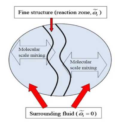
Fig. 2. Computational cell-based schematic on the EDC model. (Gran and Magnussen, 1996)

In this paper, Brandt model [20] is introduced where the first progress variable is developed depending on the intermediate combination and final product species. It is designed in such a way that it defines both constructions of dominant species at the beginning of the period and the following heat release. Since the chemical reactions occur within a thin reaction zone that is confined, it needs to be recognized. Also, as it is typically smaller than the computational grid size. In the Gran and Magnussen EDC model, the cell of computational can be divided into two subzones, which are fine structure and surrounding fluid highlighted in Fig. 2. All chemical reactions which are said to be homogenous are meant to perform in the fine structure at adiabatic and isobaric condition. At perfectly Stirred Reaction (PSR) condition, both mass and energy are shifted to surrounding fluid at the condition where turbulent mixing occurs, later transported to reactant and product of the surrounding to perform the fine structure [16]. The following equation (11) describes the size of the fine structure ξ and means residence time of the fluid inside the fine structure τ.

7 р^2 2 to. =--------

( Г - Y" )

i

т

Here, Х ^ = mass fraction of species, i (fine structure or reacting), Х 0 = mass fraction of species, i (fluid of surrounding), and т = mean residence time which is inverse of the rate of the specific mass exchange rate between fine structure and surrounding = ^.

• G.    EDC Model Extension with Temperature Variance Equation

The reaction rate of the EDC model can be evaluated using the mean temperature which is obtained by the solution of the energy equation. However, temperature variance measurement is implemented as greater interest in extending the EDC model with the temperature variance equation. By assuming weak dependency of the mean of specific heat on temperature and composition, the modelled equation for the variance is proposed as follows in the equation (12).

d PtT "2j      -     " 2

5 ⁽ p u/T )

-------+--------- д t             д x.

г

Pt id(pT ) p + — I—;— ^t J   5x

! ⁺ Cp ^t

' д ( T " 2

д x.

V - J

C d P T

+ 2 p

Here, C_p =2.86, C_d =2.0 and a_t =0.85 are termed as model constant.

From this equation derivation, an assumption of gradient diffusion has been implemented for modelling turbulent scalar flux and the assumption of simple relaxation has been implemented for modelling temperature variance dissipation rate. The last term of the above equation resembles temperature fluctuations production cause by releasing heat by chemical reaction, to>_T . To simplify, this contributed term is being assumed as negligible. The model variance shows no influence on the EDC model mean reaction rate and prepared as a post-processing model. As for comparisons between the simulation model and measured value, it can be assumed that the value of mean experimental and standard deviation from CARS can be directly distinguished with a computed value of Favre averages.

• H.    The Non-premixed Turbulent Combustion Model

The aim of modelling turbulent combustion is to perform closure to the mean chemical source term. The combustion model is divided into several categories: The model of infinite fast chemistry, Probability Density Function (PDF) models, and laminar flamelet models. In non-premixed combustion fuel and oxidiser, mixing occurs simultaneously. Therefore, non-premixed combustion with fast chemistry is beneficial to describe the mixing fraction between fuel and oxidiser. With a non-premixed (or diffused flame) model, an assumed shape of probability density function (PDF) is used to describe the turbulence chemistry interaction. Therefore, a steady flamelet approach or equilibrium is used to calculate the thermodynamics state of the fluid, as it is related to the mixture fraction. Hence, getting a robust and faster solution for any turbulent reacting flow, which is suggested for a non-premixed model, that is at or will be close to chemical equilibrium. Usually, a model like this is used for Process furnace, gas turbines and IC engine application.

• I.    The Flamelet Concept

The concept of flamelet shows the turbulent flame which is a combination of laminar, thin and one-directional flamelet structures is created within the turbulent flow field. Generally, the common laminar flame is used to shows a turbulent flow flamelet which is the term as diffusion flame of the counter flow. The following Fig. 3 shows opposed axisymmetric fuel and oxidizer jets. If there is a reduction of the distance in between the jets or there is an increment of jet velocities, the flame becomes strained and subsequently starts to deport from chemical equilibrium until extinguishment. In the experiment of laminar counterflow diffusion flame, the species temperature field and mass fraction are calculated. By having an affordable complex chemistry calculation, the governing equations and self-similar solution could be confined into one dimension.

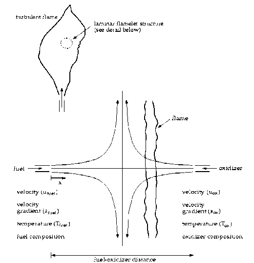
Fig. 3. Computational cell-based schematic on the EDC model. (Gran and Magnussen, 1996)

In this flame of laminar counterflow, the mixture fraction, f, x = 2D\V/\ ²starts to decrease gradually from unity level at the fuel jet to zero levels at the oxidizer jet. There are two parameters, such as strain rate and mixture fraction which are used to describe uniquely, in conditions when the species mass fraction and the temperature along the axis are plotted and initiating a physical space for mixture fraction. The scalar dissipation can be expressed as:

a s exp ( - 2[ erfc — 1 ( 2 N ) ] 2 ) x St = ------------------------------

П where the chemistry reduced and fully explained by two quantities of f and x. The complex chemistry reduction to two variables leads to pre-process of flamelet calculations that are stored in look-up tables. Hence, the computational cost reduces significantly.

The strain rate characteristic for flamelet of contra-flow diffusion is obtained from d_s = v / 2d, where, v = fuel and oxidizer fuel speed, d= distance between jet nozzles. In physical, when the flame is strained, the reaction zone width diminishes and the mixture fraction gradient at stoichiometric position increases, f = f_st. The non-equilibrium parameter is known as stoichiometric scalar dissipation. It has the dimension of s ^-1 that is term as inverse characteristic of diffusion time. Therefore, when x_st ^ 0 the chemistry terms as equilibrium however, the value of x_st increases because of the straining of aerodynamics increased of non-equilibrium. The flamelet local quenching occurs whenever x_st exceeds the critical value.

• J.    The Laminar Flamelet Model

The laminar flamelet method is proposed by Peter and Kuznetsov where the diffusion flame of the turbulent includes stretched laminar flamelet. The mass fraction of Favre-averaged for non-premixed combustion of k species has resembled in the equation (14).

∞

Y_k ( x , t ) = ∫∫   Y_k ( Z , χ _st , t ) P ( Z , χ _st , x , t ) d χ _stdz ,

where, x_st = Scalar dissipation at the surface of the flame, P ( Z, x ,,, x, t ) = Presume-PDF, and Y_k ( Z , %_s, t ) = Laminar flamelet at different strain-rates.

The limitation of the laminar flamelet is confined to the flamelet regime. In the flamelet regime, the flamelet structure integrity preserves and eddies of the turbulent do not extremely distort the flame structure. Therefore, in this regime, the flame sheet local structure equals a laminar flame to better approximation.

K. The PDF model

The joint method of PDF transport equation was proposed by Pope, where the transport equation, viscous dissipation and scalar reaction are solved. This equation does not carry any details of the result of the mixing term which requires further modelling of an unclosed term [21]. Therefore, the mixing term closure is needed. The main benefit of the joint PDF transport equation is the closure term acts in closed form and where closure model is not required. Also, it does not make any assumption of fast chemistry for non-premixed combustion and the best existing turbulent reaction flow to describe completely. It is likely to deliver closure to the misting term utilizing scalar gradients in the equation of transport at the higher cost of computation and dimensions. Pope introduced the Monte-Carlo simulation method by utilizing Lagrangian methods for reducing the cost of computation. In this method, the fluid is scattered with virtual particles. These particle evaluations are modelled and imposed the macro mixing by utilizing the method of a random walk. The scalar concentration is calculated by the use of stochastic models with micromixing. Like other turbulent models, the predictions rely on closure model quality. The foremost drawbacks of these methods are expensive computational, complex mathematical and complex mixing closure.

4.    Simulation Setup

• A.    Computational Domain and Grid

ICEM CFD Utility Meshing is used to discretize the computational domain for 2D meshing. The first block in Fig. 4. represents the injected fuel, and the second block represents hot air co-flow. As the burner is axis-symmetry, therefore 2D axisymmetric grid is being utilized. The computational domain starts from the jet exit and further down up to 41.4mm and 200 mm for both cases in the axial direction. However, the grid of radial direction is extended up to 81.8 mm.

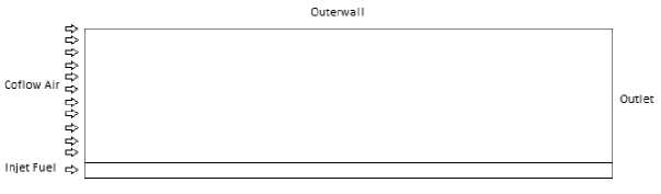
Fig. 4. Computational Domain.

These radial directions take into account where the effect of co-flow air. The grids consist of the following cells for two different meshes as a result of mesh independence. The study of grid independence was carried out for both coarse and fine mesh.

• B.    Boundary Condition

The highest axial distance of both computational domains is termed as pressure-outlet. The symmetry is termed as lateral boundary and inflow term as the burner exit. For both test study jet and co-flow at inlet boundary, the physical quantities value is set equal to tabulated values for both study cases in Table 1. The boundary conditions are applied to the flow variable are listed in the table. Fv and zG are standing for fixed volume and zero pressure gradient, respectively. The zero gradient approach is imposed for applying boundary conditions in a non-limited by the domain of the solid surfaces. When flow attains steady-state condition, the assigned outer limit turns to a streamline parallel to the flow axis, and it is numerically verified and also reaches the same velocity of the air co-flow. Table 2 shows the boundary condition mechanism applied for CFD simulation.

Table 2. Fuel and Coflow composition.

Gases	Transport species modeling of non-premixed combustion using Methane air two-step mechanism		Non-premixed combustion modeling PDF approach
	Dutch natural gas	Air	Fuel-jet	Air
N 2	0.15	0.924	0.15	0.924
O 2		0.076		0.076
CH 4	0.85		0.85

The velocity, temperature and temperature variance are highlighted in the results. The turbulent intensity is set as 10%. The kinetic energy of turbulence, k in the inlet boundary is determined by calculating the Reynold Stress of normal axial and radial components and through the assumption of azimuthal component, which is equal to radial one, i.e.,

'2         '2                    '2         '2          '2

w = v (2 k = ( u + v + w ))

The number of k and ε are expressed in term of a function of turbulent intensity (I_t) and characteristic length (L_t) respectively. The values are calculated by following correlations:

k = 1.5( ul_t )²

e = 0.1643 k ² ( L_t ) - ¹

The initial values are needed to be appropriately determined for ensuring stability at the beginning and adequate accuracy to solve conservation equations. The initial boundary condition of species is followed for both EDC model with DRM 22 and PDF Flamelet approach model with GRI 3.0 is tabulated in Table 2 incoming flow mass fraction extracted from Oldenhof et al experiment of DJHC burner. It is noted that the initial value of mass fractions for N 2 and O 2 are imposed rather than other species. It represents that air is initially present in the computational domain. Also, turbulence properties of co-flow air are set according to intensity and characteristics length (listed in the table) when the air motion in the computational domain begins.

5.    Results and Discussions

• A.    Grid Independency

  The grid independence investigation is being carried out for verification of the result prediction for both test cases represented in Fig. 5. Auto-ignition is taken place at very lean condition because of reduced oxygen composition in the co-flow. The turbulent co-flow is also strongly affecting the chemical reaction; therefore, turbulent chemistry plays a vital role in the MILD-combustion regime. However, proper flow prediction and mixing are necessary to run a successful model. The test case with Re = 8800 was taken as a grid independence study represent having the highest jet velocity.

Fig. 5 shows the result prediction, which is calculated from two different grids for the mean axial velocity of at downstream x = 30mm and the comparison to the experimental value. However, the simulations with different grids give a good agreement of results. It is noted that the injecting rate of the jet is a little bit under-predicted as visible in Fig. 5 Since both meshes have the same results, therefore, the coarse mesh was selected for the rest of the result of the simulation.

■ Experimental

^^  ■ Coarse mesh result

^^  ■ Finer mesh result

Radial direction (mm)

Fig. 5. Grid dependency

• B.    Velocity Statistics Prediction

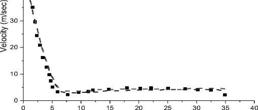
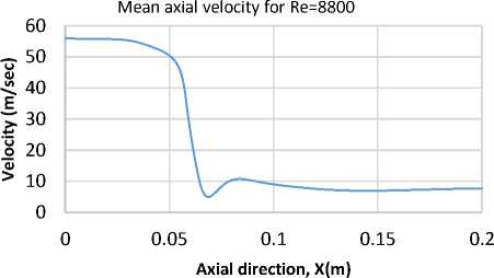
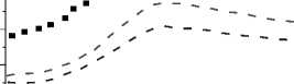
  The estimation of mean velocity and turbulent kinetic energy for the simulated model of DJHC-I burner for both Reynolds number of 4100 and 8800 are being compared with existing experimental data. The following Fig. 6. show the centre-line of mean velocity profile in the direction to axial (U _x ) and turbulent kinetic energy (k) for Reynolds number of 4100 and 8800 for steady diffusion flamelet PDF model.

Sudden axial velocity drop is observed for both Reynolds number as the value of mean density decreases as well as convection decreases. But at this point, the diffusion of counteraction is found higher for both Reynolds number highlighted in the following in Fig. 6.

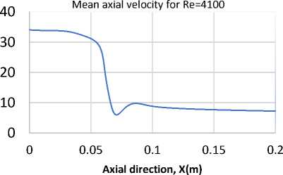
Fig. 6. Mean velocity profile along centre-line for Re=4100 and 8800 for steady diffusive flamelet PDF approach.

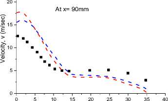
The turbulent kinetic energy for both Reynolds number at axial direction follows the same trend of fluctuations. For the same respect, the DJHC burner is modelled by suggesting an EDC concept model with GRI Mech 3.0 chemical mechanism for fuel I type. The radial velocities at different downstream locations start from (x = 30 mm, 60 mm, 90 mm, and 120 mm) for Reynolds number of 4100 is studied using steady diffusive flamelet pdf approach and EDC approach and compared with available experimental data of DJHC burner in following Fig. 7.

25 -Г

Experimental

Flamelet PDF Approach model

EDC model

Е

At x= 30mm

10     15    20     25     30     35    40

Radial distance, r (mm)

10      15      20      25

Radial distance, r (mm)

30      35

Radial direction, r (mm)

Radial distance, r (mm)

Fig. 7. The centreline mean velocity of radial profile at different down-streams positions (x=30mm, 60mm, 90mm, and 120mm) for Re=4100 using a steady diffusive flamelet PDF approach and EDC model.

It is detected that the centreline profile of mean axial velocity at x = 30 mm is in good agreement with the experimental one for both models, though, subsequently, the centreline peak values trend towards under-prediction at later downstream. While the overall result’s prediction in the mixing layer shows good reasonable agreement in the radial direction, it appears some over-estimation in radial velocity at various downstream is associated with the overestimation of mean temperature.

In this case, the value of mean density is being decreased, which leads to a decrease in the value in convection at the axis. However, at the same time, the diffusion of counter-acting is becoming higher. It means the diffusive force of fuel feasts the jet promptly in the radial direction, causing under-prediction in the value of the centre line. Reynolds normal stress u'u' is an essential quantity for describing mixing momentum between fuel and co-flow air. The two sets of data are calculated from different models with different mechanisms and a complete flame traverse. It is found both symmetry side axis has a slightly different experimental profile.

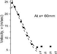
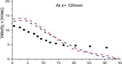
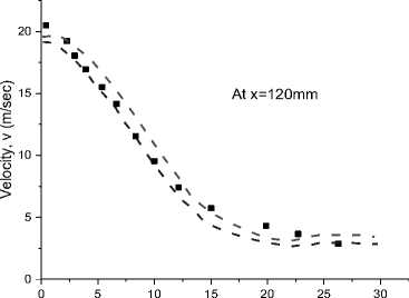
The following Fig. 8 shows the radial profile of mean radial velocity at various downstream locations from the jet exit for Re = 8800 which is compared with the turbulent model in the flamelet PDF approach and the EDC model with GRI 3.0 and DRM 22.

0Т-----------------------'-----------------------1-----------------------1-----------------------1------------------------1-----------------------1-----------------------1-----------------------1-----------------------1------------------------1-----------------------1-----------------------1-----------------------1-----------------------1

0      5      10      15     20     25     30     35

Radial distance, r (mm)

At x= 60mm

0       5       10      15      20      25      30      35

Radial distance, r (mm)

Radial distance, r (mm)

Fig. 8. The centreline mean velocity of radial profile at different down-streams positions (x = 30 mm, 60 mm, 90 mm, and 120 mm) for Re = 8800 using flamelet PDF approach and EDC model with GRI 3.0 and DRM 22 mechanism.

Fig. 8 shows under-prediction of centre-line mean velocity at the radial direction from 60 mm to 120mm downstream location, where there is a good agreement of results for x = 30 mm. There is a good agreement of results for x = 60 mm from the flame, but it tends to deviate under-prediction at the far end of the flame because of Reynolds stress.

Both Fig. 7 and Fig.8. show good agreement results prediction for both cases of Re = 4100 and 8800, but the flamelet PDF approach has a slightly better agreement. The velocity contour calculated from both simulations is illustrated for both the Reynolds number in Fig. 9.

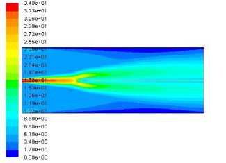
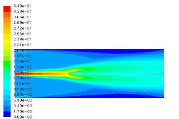
Fig. 9. Velocity contour for simulated DJHC-I burner using the flamelet PDF approach and EDC model with GRI30 and two steps mechanism respectively.

• C.    Temperature Statistic Prediction

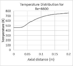
The temperature predictions for both Reynolds's numbers were determined. The temperature profile for both Reynolds numbers at the axial direction is illustrated in Fig. 10.

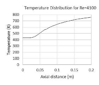
Fig. 10. Temperature profile for both Re=4100 and 8800.

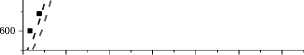
Extensive differences in the profile of mean temperature are observed between using two models and experiment one. The mean temperature profile for both models with Re = 4100 and 8800 at different downstream are compared with the experiment in Fig. 11 and Fig. 12

■ Experimental

Flamelet PDF approach EDC model

1200 ф .

"S 1000

At, x=60mm

0       5       10      15      20      25      30

Radial distance, r (mm)

400 n------------------1---------1---------1---------1---------1---------'---------1---------'---------1---------1---------1---------1---------r

0      5      10     15     20     25     30     35

Radial distance, r (mm)

Radial distance, r (mm)

Fig.

11. The center-line

compared.

$ 1400

Е .

1000 -L ^

600 П-------------'-------------1-------------'-------------1-------------'-------------г

0              10              20              30

Radial distance, r (mm)

mean temperature profile at different downstream for Re = 4100 using two different models and experiment which are

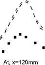
At, x=90mm

At, x=120mm

2        '

Е

10              20              30

Radial distance, r (mm)

10               20               30

Radial distance, r (mm)

Fig. 12. The center-line mean temperature profile at different downstream for Re = 8800 using two different models and experiment which are compared.

Two problems appear where the first problem conducts on predicting a peak temperature by SKE at r = 7.5 mm and 12 mm in the mean temperature radial profile at the downstream location 30 and 60mm. Where the peak temperature profile at 60 mm in the simulation reflects too early ignition and the second problem shows that SKE performs under-prediction on mean temperature (r>25mm for x = 30mm and r>12mm for x = 60mm). The standard k-ε model predicts over-predicts means temperature at a large scale of r (r>15 mm for x = 60mm for both Re and x = 90, 120 mm for Re = 4100). On the other hand, it also under-predicts means temperature at a large scale of r for x=90 mm and 120 mm. It is a matter of measurement error that needs to be compared with the results of the k-ε model for future interests. It happens because SKE gives entrainment’s over-prediction by bringing too much cold air from the surroundings. But experimental study later proves a decrease in lift-off height with the increased value of Reynolds number. The standard k-ε model is providing an under and over-prediction for entrainment for Reynolds number = 4100 and 8800, respectively through acquiring much cold air from surroundings. The over prediction of mean temperature occurs due to maintaining the balance between temperature fluctuation of production and destruction. After all, the experimental data gives an idea of decreasing lift-off height with the crease of Reynolds number. It is also explained the effect of co-flow entrainment from the surrounding of the fuel jet in a radial means temperature radial gradient in the co-flow. The crucial disadvantages of the standard k-ε model for better prediction of the mean temperature of the radial profile in the outer region can be neutralized, focusing on the results of other turbulence models in the future.

As the mixing momentum is being well described, the enthalpy can also be characterized by the SKE model. The possible deviation of results of mean profile temperature cannot be caused by jet and co-flows mixing; instead, it can be related to the combustion description process. The asymmetry in the measurement of the outer region less than 25mm is needed to be concentrate while comparing the prediction data, especially up to 9 0mm. As ignition has been predicted early because the peak temperature is at the shear layer of the outer edge in the stoichiometric zone. The temperature peaks appear in the region where fuel and co-flows are present in the proportion of stoichiometric from the above figure. So, the temperature is well predicted for x = 15 and x = 30, but from x = 60, it tends to be over and under predicted along the shear layer inner edge. Also, there are peaks in the radial temperature profile (10>r>20) as a result of an overestimation of the rate of mean reaction in the EDC model, but there is less peak in the flamelet PDF model. It is also proved there are no substantial differences in temperature prediction using different chemical mechanisms and different turbulence modeling. Overall, it is observed that the EDC model shows better agreement over the Flamelet PDF approach. As the results are not converging properly, so still there is a need for further convergence. At the MILD regime, the reaction and flow are not fully developed. However, the combustion is stabilized near the downstream region for which the results with downstream, x = 60 mm gives good agreement but at the far downstream region, results are still vague, which needs more converge results.

• D.    Effect of Reynolds number on Lift-off Height Prediction

In the DJHC flames experimental study, Oldenhof et al. have pragmatic that the height of first ignition kernels declines with the increase of Reynolds number of fuel jet. As the increase of entrainment links with the increase of fuel jet velocity being coupled with a positive radial temperature gradient located at x = 0. Well, prediction is performed for the flow field with entrainment employing the standard k-ε model for both the Steady Diffusion Flamelet model and EDC approach model available in ANSYS FLUENT. The model combustion reaction mechanism is considered to calculate the mass fraction of the species and to identify its contour approximation of mean stoichiometric where fuel and are engaged as base streams by inputting mean mass fraction and investigate the contour near stoichiometric to approximate the mass fraction. The mean mass fraction of OH is considered to monitor the lift-off height that linked to the presence of probability of pocket flame. Typically, the pocket flames are at the point where the OH mass fraction is 1e-3.

Fig. 13 identifies the locations (arrow sign) of the OH mass fraction with a value of 1e-3 where the possible pocket flame exists for two different Reynolds jet fuel flames. The figure comparison shows the lift-off height increases with the increase of jet Reynolds number.

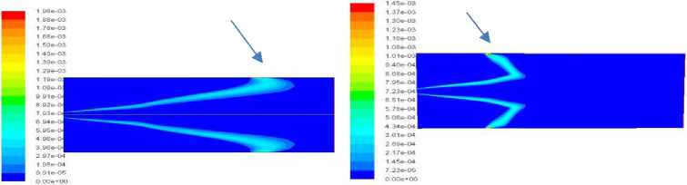
Fig. 13. The mass fraction contour of OH for Re=4100 (left) and Re=8800 (right).

Fig. 14 clarifies the increase in the lift-off height with increases in Reynolds number, Re for DJHC burner. It was observed that due to fast mixing in between the incoming hot gases and fuel jet, the reactions accelerate, and autoignition length minimizes where similar observations were performed by De et al. [7]. This study shows the proposed tabulate chemistry model ability on turbulence chemistry of the stochastic field’s interaction for considering the case with mixing of multi-stream.

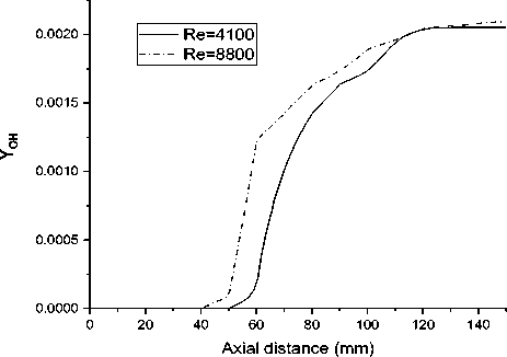
Fig. 14. The mass fraction contour of OH for Re = 4100 (left) and Re = 8800 (right).

6.    Conclusion

The paper comprises the numerical investigation of MILD combustion behaviours of DJHC burner with a co-flow of 7.6% oxygen for Reynolds number 4100 and 8800. Two different turbulent-chemistry interactions model named Eddy Dissipation Concept (EDC) model with chemical mechanism GRI mech 3.0 and Steady Diffusion Flamelet model with DRM 22 were applied to study the capability of numerical study for experimental data calculated by Oldenhof et al . [12]. The prediction of mean radial velocity and temperature field for both simulated models with different Reynolds number offers good agreement with experimental data at a near downstream location. However, at a high stream location, the results show different behaviour compared to experimental data. One of the best advantages found of better prediction of mean velocity and temperature profile at downstream position smaller than 60mm. The outer region cold air co-flows entrainment from the surrounding acts as a vital role which is predicted in this model. As expected, the standard k-epsilon model gives sensible result for this round jet system but modified the k-epsilon realizable can be accountable as for future reference work. The mean temperature prediction provides expected deviations from that of experiment result at a near downstream location. The mean temperature profile in radial direction illustrates a peak because of occurring early ignition. It proves this model underpredict the height of lift-off at a low computational cost. Therefore, the decrease in lift-off height resulted in increasing the jet exit velocity. The numerical results explain the application of implicit conclusion in the framework of MILD combustion, with the choice of investigation of different approaches in the realistic configuration depending on different Reynolds number and chemical mechanism. The further study involves investigating the behaviour EDC concept model with a more computational cost that would perform exploration of better agreement with experimental results. The future goal is an in-depth study of the formation of NOx and SOx composition at different axial location in the combustion process and the starting enthalpy study to perform wall heat losses in a cost-benefit assessment.

Acknowledgement

The authors acknowledge the financial support from the Bangladesh Bureau of Educational Information and Statistics (BANBEIS), Ministry of Education, Bangladesh (GARE Project No.:- PS2017594; 2018-2021), Ministry of Science & Technology, Bangladesh (Project No.:- EAS-448 and EAS-450;