On a GARCH Model with Normal Scale Mixture Innovations

The volatility of returns has important theoretical and practicality meaning in the applications of risk management and asset pricing. Volatility clusters (i.e. Volatility may be high for certain periods and low for other periods) are commonly seen in financial time series. Also, financial time series, which marginal distribution have higher excess kurtosis, typically exhibit the feature of heavy tail.

In the past two decades, various models have been proposed in order to describe these features. Among them, the generalized autoregressive conditional heteroscedastic (GARCH) model of Bollerslev (1986) has been proven to be a powerful one in capturing the empirical features. The GARCH(p,q) model is defined as

X = e^h t ,

• <               q                P                                                                                                   (1)

ht=«0+E ajX- j+E Piht - i, te N, j=1                 i=1

* Corresponding author.

Where p , q — 0 are integers; a >  0 , a , в — 0 are constants , to ensure positivity of h_t , for all t ; ^ are i.i.d. with zero mean and unit variance; and ^ q a + ^ p в <  1, to ensure covariance stationarity. The random variables ^ are called the innovations and usually assumed to be standard-normal. When p = 0 , the model reduces to the ARCH model of Engle (1982).

Unfortunately, the normal GARCH models seem to be much thinner than the tails apparent in the data, that is to say, the normal GARCH model can’t interpret all the excess kurtosis. A popular candidate is the GARCH-t model (Bollerslev, 1987), which used the t distribution innovations assumption. However, the discussion of GARCH process excess kurtosis makes some senses only if the freedom of t innovation distribution greater than 4, otherwise, the ability of capture the tails behavior for the model will be cut down. Other papers dealing with alternative mixture GARCH models are Wong and Li (2001), Zhang (2006).

In the statistics literature, mixtures of distributions have been widely used in modeling of heavy-tailed distributions, and noticed the fact that we can obtain heavier tail marginal distribution than the innovations’ distribution by the GARCH process, we considered a natural extension of Bollerslev (1986) by using NSM innovations instead of normal innovations in this paper.

The rest of this paper is organized as follows. Section 2 presents the GARCH model with mixture normal innovations and illustrates its flexibility in capturing the characteristics in financial time series. Section 3 describes the parameters estimation procedure using EM algorithm for the model. Section 4 illustrates our procedure for the log return series of the Shanghai Market Index which is a clear example of a series large kurtosis and extreme returns.

• 2.    The GARCH model with normal scale mixture innovations

  • 2.1.    Normal Scale Mixture Distribution

Mixture Models are a type of density model which comprise a number of component functions, usually Gaussian. The two component normal scale mixture (NSM) distribution under considered is defined by f (y; ст2,2, p) = pf (y) + (1- p)f, (y)

Where f ~ N (Q, _CT ²) , f ~ N(0,a²/ 2 ) and 0 < p , 2 <  1.

An alternative definition of у ~ NSM ( 2 , p ) as

N (0, ст ²)    withprobability p ,

Y ~ ^

N (0, ^ ²/ 2 )  withprobability 1 - p .

This family was introduced to model a population which follows a normal distribution except on those few occasions where a grossly atypical observation is recorded.

We can deduce an important property of NSM distribution concerned on its kurtosis by calculating some expectations.

THEOREM 1. Suppose Y ~ NSM ( 2 , p ) , 0 <  p , 2 <  1 . Then the kurtosis of Y is given by

K, = 3 + K > 3 , where K = 3p(1 - p)((12) -1)2 '     [ p + (1 - p),2]2

.

Proof Since E ( Y ²) = f y ² f ( y ; p , 2 ) ^y

-да

= ^р y- ^ ( y) ) dy + (1 ^- р )р — J= ^ () dy

■ -” C C          J-“ c/ XXC/ 4Х

Г+”    1                хГ” 722   1

= ^р t 1 ² -ф⁽t DCT dt i + (1 ^- р )l t ₂--- Т (=Ф1.t 2)р= d 2

J-”    с               J-” x c/XxXX

= pc ² + (1 - p )^-, and E(Y ⁴⁾ = [ y ⁴ f ⁽ y ; p , ^{X )}dy

X

= ^p ”y- ^{Ф (} y )dy + ^{(1 -} P ) j"⁰⁰ —r^( ^ф(—pi= ) dy

J-” с c         J"” c4xc4x

+”      1                     Г+”  c4    1

= p\ t 3 ^{c   ф} t 3 ) ^{c dt} 3 ^{+ (1 -} P )f t 4         -^ф t 4H7 ^dt 4

• J ■    c             J-”  X c4xXx

• 2.2.    The Definition of GARCH Model with Normal Scale Mixture Innovations

= 3 p ( c ²)² + 3(1 - p )(c²/ X )², Thus we have к - E ⁽ Y ) - ^{3 p + 3(1} - ^{P )(1 X )}

Y   [ E ( Y ²)]²     [ p + (1 - p )/ X ]²

3p+3(1 - p )(V X)2 _3 , [p + (1 - p)/X]2.

= 3 + 3p^{(1 -} p ⁾⁽V ^X - 1⁾² >  3. [ p + (1 - p )/ X ]²

We consider the innovations in equation (1) follow normal scale mixture distribution, that is ^ ~ NSM ( X , p ) , so we have the GARCH(p,q)- NSM ( X , p ) model defined by

Xt = Eclht, qp

‘ h t = « 0 ■ Z ^a j^X2 j ⁺ Z P i h t - i ,                                                              ⁽⁴⁾

j = 1                   i = 1

^ i.i . d . ~ NSM ( X , p ), t e N ,

Where p , q >  0 are integers; 0 <  X , p <  1 ; a = ( a , — , ^ ) T and в = ( A , ^ , в ) T follow the restrictions, a >  0 , a , A >  0 are constants , 'Z ^? _j a + ~Z P-! A <  1 ; and c ² = 1/ ( p + (1 - p )/ X ) , so that Var (£_t ) = 1 .

According to the definition, the innovations ^ are generated from a normal distribution with variance c¹ with probability p , or from a normal distribution with variance c²/X with probability 1 - p . We also impose the condition that the probability p is restricted to the interval (0.5, 1) to ensure that the component with largest number of elements is the one with smallest variance.

The reason of using the NSM distribution to model the innovations instead of a Student’s t distribution are as follows. If ^ follows a Student’s t distribution with V degrees of freedom, thenKK = 6/v - 4 . Note that the second and fourth moments of Xt only exist if v > 4, implying that the excess kurtosis Kg should be positive. However, in practice, the degrees of freedom parameter, v is either fixed to be larger than or equal to 5, in which case the implied kurtosis of the estimated model does not match the observed kurtosis, or it is estimated, in which case its estimate is usually smaller than 5, and the estimated excess kurtosis does not exist.

• 3.    Estimation via EM algorithm

  In this section, we discuss the estimation of the parameters of a GARCH model with normal scale mixture innovations using the EM algorithm (Dempster et al., 1977). Suppose that the observed time series r = { r , . , r_T } is generated from the following model (5).

^ i.i.d . ~ NSM ( Я , p ) t = 1,..., T .

where Mt is a stationary mean process of {r} , other notations are same as (4), (5).Let z = {z1,..., zT} be the unobserved indicators, where zt equals to 1 if 8t ~ N(0,°2) and equals to 0 if ^ ~ N(0, °2/Я).

Then, conditional on these indicators, we have that,

~

if zt = 0, if Zt = 1,

t = 1, . , T .

We call r the incomplete data with missing data z . Let 6 = (Я, p,aT, в )T be the parameter vector of model (5). The likelihood is given by

T

L (6| r, z ) = П t=C+1

P    r - M

ф|    /

° V h I ° V h

(1 - p) 4x ° hFi

^{( r} t ^- M t ) V ^я ^sjh

where c = max( p, q); ф(-) is standard normal density function, For simplicity, we denote that f11=-^.

^ r t - M t

' Vh" ( ° hK

Уя

, ^f - 1      ^ф

^ V h t

⁽ r ^- Mt ) V ^я

^ hpit

, ft = Pf\t + (1 — P ) f t , then the joint density of r

and zt will be g(rt, zt ;6^ = [pft ]zt [(1 - p)ft J zt and the conditional distribution of zt conditional on r given by

P (zt= 1|rt;6) = pf,   P (z= 0 r;6) = (1 - p) ff , t = 1,., T(8)

ff

According to (8), we can obtain the (conditional) log-likelihood as follows

T l =^ in g(r, z ;6)

t = c + 1

The iterative EM procedure for estimating the parameters by maximizing the log-likelihood function (9)

consists of an E-step and an M-step. These steps are described in the following.

E-step: Let O^⁰ be the value specified initially for 6 , Then on the (m)th iteration of the EM algorithm, the E-step requires the computation of the conditional expectation of l given z , using 6 m ^{- 1)} for 6 , which can be written as

T

Q (6O.....)  X Ец, -)Иg (г z^) ]

t - c+1     1

T Г    m ^{- 1)} f^{( m - 1)}                      Dm^{m - 1)}1 f^{( m - 1)}

- X ^P Л mf )   ^ln( P f t ) + ^{(   P} A m - ^{) f} 2 *   !n(d - P ) f 2 1 ).

t - c+1 _    ft                                  ft_ ft(m-1) — (m(m-1) (mm-1) ry(m-1)T (mm-1T) AT      y(m-1) —       m-1)A      f(m-1) — f (ft-m-1)A where 6     - (A .p ,a      , p      )   .  ft     - ft(O    ) .  ftt    - f1t(O)

.f 2m -" - f 2 , ( 6 m ^{- 1)} ) , f\- f( 6 ) . f t - f 1, ( 6 ) , f 2 1 - f _: t ( 6 ) ;

M-step: The M-step on the (m)th iteration requires the global maximization of Q ( 6 , 6⁽ m ¹⁾ ) with respect to 6 over the parameter space Q to give the updated estimated 6 ^{m )} , which can be obtained by solve the equations ^d Q( ^{6 ,} °^ m -") - 0 d 6

The estimates of the parameters 6 are obtained by iterating the E and M steps until convergence.

• 4.    An example

  The word “data” is plural, not singular. In American Eng As an illustration, we select the Shanghai stock market daily closing index from December 16th, 1996, to April, 27th, 2007 (2500 observations). The

computational results and the analysis of the real data example in this section have been carried out by means of various routines written by the author in MATLAB (The MathWorks, Inc.). The sample mean, variance and kurtosis coefficient of the log return series are 5.30 x 10 - 4 ,2.46 x 10 - 4 , 8.97 respectively. Note the large sample kurtosis of the returns.

We first fit a normal GARCH model to the log return series , in which innovations assumed to be standardnormal. It is also the best model in the sense that it minimizes the AIC and BIC over all the normal GARCH models. The estimated model is given in the following (11),

'r_t - 0.34745 г , - 3 + X_t , X - ^ h^ ,

(1.7085)

_< h, - 6.2585 x 10 ^{- 6} + 0.1162 X2. , + 0.8647 h,__p                                                          (11)

• (7.4987)       (16.4347)   (144.4248)

^ i.i.d . ~ N (0,1). t - 1,2,..., 2499,

_ AIC -- 1.4181 x 10 4 , BIC -- 1.4158 x 10⁴.

where the numbers in brackets are T statistics values. According to the upper graph in Fig.1, in which displays a quantile-quantile plot of stand residuals versus standard normal distribution in model (11), it is not difficult to find that model (11) is poor in capturing the heavy-tailed features in the data.

The inadequate of model (11) suggest us consider a GARCH model with heavy-tailed innovations distribution for the data. A candidate can be GARCH model with normal scale mixture innovations which provided in (4). The GARCH model with normal scale mixture innovations can be estimated using the EM algorithm in part 2 for detail and given in the following (12),

'r = 0.06550r- + X,, X, = еДк,, к = 1.01502x10-6 + 0.14239X2. + 0.71540к ., —1                    t-i,

[ N (0,0.77924 2 )        , with prob. 0.81188,

• < е i.i.d . ~ i                                                                          .

• 5.    Conclusion

[N(0,0.779242 / 0.22531), with prob. 1 - 0.81188, t = 1,2,...,2499,

AIC = - 1.423 7 x 10 4 , BIC = - 1.4202 x 10 4 .

For purposes of comparison the two candidate models, we plot the quantile-quantile plot of stand residuals versus innovations’ distribution each other and put together in Fig 1. Obviously, the GARCH model with normal scale mixture innovations is much better than the normal GARCH model for fitting this series. On the other hand, the BIC and AIC model selection criteria also give the same choice.

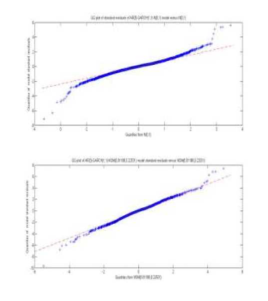
Fig. 1 PP plots of the two comparative models

The proposed GARCH model with normal scale mixture innovations provides an extension of the standard GARCH model. Its tail behavior can be thicker than that of the normal GARCH model. The GARCH Model with Normal Scale Mixture Innovations may be worth considering if accurate modeling of the tail is important in such applications like the estimation of value-at-risk.

Acknowledgements

I would like to express my deep and sincere gratitude to my supervisor, Mr. Zhang Zhiqiang, Professor of the Department of School of Finance and Statistics, East China Normal University. His wide knowledge and his logical way of thinking have been of great value for me. His understanding, encouraging and personal guidance have provided a good basis for the present thesis.