On Applications of a Generalized Hyperbolic Measure of Entropy

Published Online June 2015 in MECS

The main use of information is to remove uncertainty and main objectives of information theoretic studies are:

• •    To develop new measures of information and their applications

• •    To develop entropy optimization principles

• •    To develop connections and interrelations of information theory with other disciplines such as science, engineering, management, operation research etc.

• •    Exploration of role of additional parameters in generalized information/divergence measures.

Entropy is central concept in the field of information theory and was originally introduced by Shannon in his seminal paper [1], in the context of communication theory. The entropy of an experiment has dual interpretations. It can be considered both as a measure of the uncertainty that prevailed before the experiment was accomplished and as a measure of the information expected from an experiment. An experiment might be an information source emitting a sequence of symbols (i.e., a message) M = {s1,s2,...,sn}, where successive symbols are selected according to some fixed probability law. For the simplest kind of source, we assume that successive symbols emitted from the source are statistically independent. Such an information source is termed a zero-memory source and is completely described by the source alphabet and the probabilities with which the symbols occurP = {P1,p2,...,pn} . We may calculate the average information provided by a zero-memory information source using several entropies. The Shannon Entropy [1] is a well-known and highly used measure of information.

Consider a set E of mutually exclusive events E i ( i = 1, ..., n ) each of which has the probability of occurrence p i , so that the p i s add up to unity. The information content of the occurrence of event E , is defined [1]:

Inf ⁽ E i ) = - log Pi = log—.

pi

The expected information content of an event from our set of ‘n’ events, the entropy of the set E, is defined [1]:

nn

H ^{( P} ) = ^ Pi Inf ⁽ E i ) = ^- ^ Pi log Pi .         ⁽¹⁾

i = 1                           i = 1

H ( P ) is always non negative. Its maximum value depends on ‘n’. It is equal to log n when all p i are equal. H ( P ) is known as Shannon Entropy or Shannon’s measure of Information. In 1961, to add flexibility to Shannon’s measure, Renyi [2] proposed a one parametric generalization of Shannon’s measure. After Renyi, many one, two, three and four parametric generalizations have been proposed by the scholars in the field of information theory.

Bhatia and Singh[3] proposed a one parametric hyperbolic measure of entropy as follows:

n

H a ⁽ P ) = —T——■ V Pi sinh a log Pi), a > 0.   (2)

slnh( a ) ”

llm^ H a ( P ) = H ( P ).                     (3)

Thus the Shannon measure is the limiting case of the measure proposed in Eq.(2).

After the initiation of fuzzy theory by Zadeh[4], the concept of fuzziness has influenced almost each and every branch of research. The influence of fuzzy theory in the field of information theory gave birth to non-classical information theory. De Luca and Termini[5] proposed a measure of fuzzy entropy corresponding to probabilistic entropy of Shannon given by

n

H ( A ) = - - V ⁿ ^ I

P a ⁽ x i ^)log P a ⁽ x i )

+ ⁽1 ^- P a ⁽ X i )) log⁽l ^- P a ⁽ X i ))

some applications of generalized hyperbolic measure of probabilistic entropy (Eq.(2)) and generalized hyperbolic measure of fuzzy entropy (Eq.(5)) have been presented.

This paper is organized as follows: In Section II, super additivity and scalability of generalized hyperbolic information measure (2) are investigated and its application in certain situations is discussed. Section III presents a new model for mutiple attribute decision making using generalized fuzzy entropy. Section IV contains concluding remarks.

II.Application of Generalized Hyperbolic Information Measure

For notational convenience, let us call the entropy measure proposed in Eq.(2) as hyperbolic entropy (hyp entropy) and denote it as where, A is a fuzzy set and A(xi) is membership value of xi in A.

After De Luca and Termini many generalized versions of this fuzzy entropy have been proposed. Bhatia et al. [6] proposed a one parametric generalized hyperbolic measure of entropy as follows:

H hyp ( P ) =

slnh( a )

n

V p_i slnh( a log p_t ), a >  0 .

i = 1

H a ( A ) =

slnh( a )

n

V P a ⁽ X i ) ^{slnh( a} log P a ⁽ X i ))

i = 1

n

+ V ^{(1 -} P a ⁽ Xi )) ^slnh( a logfl ^- P a ⁽ X i »)

i = 1

llm a ^ o H a ( A ) = H ( A ).                        (6)

The real number α is associated with the non extensiveness of the system.

The concepts of entropy and fuzzy entropy have been extensively utilized in numerous applications in science, engineering and management[7,8]. In the present paper,

Many one parametric measures are suggested in literature. But from application point of view it has been observed that most of the applications revolves around Shannon entropy[1], Renyi entropy[2], Havrda-Charvat entropy(HC)[9] and Tsallis entropy[10]. Shannon entropy[1], Renyi entropy[2] are additive and their application is suitable for extensive systems. On the other hand, Havrda-Charvat entropy [9] and Tsallis entropy[10] are sub additive and their application is suitable for non-extensive systems. The Hyperbolic entropy proposed in Eq.(7) is compared with Renyi entropy[2] and Havrda-Charvat entropy[9] for arbitrarily chosen eight complete probability distributions and different values of parameter α. For comparison, all of three entropies have been normalized.

Table 1. Values of normalized Renyi, Hyperbolic and Havrda-Charvat Entropies at hypothetically choosen eight probability distributions at α=0.1

	α=0.1			Normalized Entropies α=0.1
Pi	Renyi	Hyp.	Havrda-Charvat	Renyi	Hyp.	Havrda-Charvat
P 1	2.29	2.08	3.66	0.991	0.930	0.983
P 2	2.31	2.24	3.73	1.000	1.000	1.000
P 3	2.28	2.02	3.63	0.985	0.901	0.973
P 4	2.28	2.05	3.64	0.987	0.914	0.975
P 5	2.28	2.02	3.64	0.988	0.903	0.977
P 6	2.30	2.13	3.68	0.993	0.950	0.987
P 7	2.30	2.16	3.70	0.997	0.967	0.994
P 8	2.31	2.18	3.71	0.997	0.972	0.995

Table 2. Values of normalized Renyi, Hyperbolic and Havrda-Charvat Entropies at hypothetically choosen eight probability distributions at α=0.4

	α=0.4			Normalized Entropies α=0.4
P i	Renyi	Hyp.	Havrda-Charvat	Renyi	Hyp.	Havrda-Charvat
P 1	2.20	2.38	2.91	0.966	0.945	0.949
P 2	2.28	2.52	3.07	1.000	1.000	1.000
P 3	2.16	2.31	2.82	0.948	0.919	0.922
P 4	2.17	2.34	2.85	0.954	0.929	0.930
P 5	2.17	2.32	2.85	0.954	0.924	0.930
P 6	2.22	2.41	2.95	0.975	0.960	0.961
P 7	2.25	2.45	3.00	0.986	0.975	0.979
P 8	2.26	2.47	3.01	0.989	0.983	0.983

Table 3. Values of normalized Renyi, Hyperbolic and Havrda-Charvat Entropies at hypothetically choosen eight probability distributions at α=0.5

	α=0.5			Normalized Entropies α=0.5
Pi	Renyi	Hyp.	Havrda-Charvat	Renyi	Hyp.	Havrda-Charvat
P 1	2.18	2.57	2.72	0.959	0.956	0.942
P 2	2.27	2.69	2.89	1.000	1.000	1.000
P 3	2.13	2.52	2.63	0.938	0.935	0.912
P 4	2.14	2.54	2.66	0.945	0.942	0.922
P 5	2.14	2.53	2.66	0.944	0.939	0.920
P 6	2.20	2.61	2.76	0.969	0.968	0.956
P 7	2.23	2.64	2.82	0.983	0.980	0.975
P 8	2.24	2.65	2.83	0.986	0.984	0.980

Table 4. Values of normalized Renyi, Hyperbolic and Havrda-Charvat Entropies at hypothetically choosen eight probability distributions at α=0.7

	α=0.7			Normalized Entropies α=0.7
Pi	Renyi	Hyp.	Havrda-Charvat	Renyi	Hyp.	Havrda-Charvat
P 1	2.13	3.19	2.41	0.946	0.994	0.933
P 2	2.25	3.20	2.58	1.000	1.000	1.000
P 3	2.07	3.18	2.33	0.920	0.993	0.902
P 4	2.09	3.18	2.36	0.930	0.994	0.914
P 5	2.08	3.18	2.34	0.925	0.991	0.908
P 6	2.16	3.19	2.45	0.960	0.996	0.951
P 7	2.20	3.19	2.50	0.976	0.996	0.970
P 8	2.21	3.19	2.52	0.981	0.996	0.976

Table 5. Values of normalized Renyi, Hyperbolic and Havrda-Charvat Entropies at hypothetically choosen eight probability distributions at α=0.75

	α=0.75			Normalized Entropies α=0.75
Pi	Renyi	Hyp.	Havrda-Charvat	Renyi	Hyp.	Havrda-Charvat
P 1	2.12	3.39	2.34	0.943	1.007	0.932
P 2	2.24	3.37	2.51	1.000	1.000	1.000
P 3	2.06	3.42	2.26	0.917	1.015	0.901
P 4	2.08	3.42	2.29	0.927	1.014	0.913
P 5	2.07	3.40	2.28	0.921	1.010	0.906
P 6	2.15	3.39	2.39	0.958	1.007	0.950
P 7	2.19	3.37	2.44	0.974	1.001	0.969
P 8	2.20	3.37	2.45	0.978	1.000	0.975

Table 6. Values of normalized Hyperbolic Entropies H hyp (P 1 P j ),j≠1 for hypothetically chosen eight probability distributions

H hyp ( P 1 P 2 )	H hyp ( P 1 P 3 )	H hyp ( P 1 P 4 )	H hyp ( P 1 P 5 )	H hyp ( P 1 P 6 )	H hyp ( P 1 P 7 )	H hyp ( P 1 P 8 )
4.430041	4.197412	4.226259	4.202577	4.208789	4.352488	4.364985

Table 7. Values of normalized Hyperbolic Entropies H hyp ( P 1 )+ H hyp ( P j ),j≠1 for hypothetically choosen eight probability distributions

H hyp ( P 1 )	H hyp ( P 1 )	H hyp ( P 1 )	H hyp ( P 1 )	H hyp ( P 1 )	H hyp ( P 1 )	H hyp ( P 1 )
H hyp ( P 2 )	H hyp ( P 3 )	H hyp ( P 4 )	H hyp ( P 5 )	H hyp ( P 6 )	H hyp ( P 7 )	H hyp ( P 8 )
4.321248	4.100226	4.127745	4.104282	4.311766	4.246897	4.258633

Let

P = ( 0.1,0.2,0.05,0.3,0.35 ) , P 2 = ( 0.1,0.22,0.23,0.31,0.14 ) ,

P₃ = ( 0.03,0.32,0.09,0.22,0.34 ) ,

P ₄ = ( 0.11,0.21,0.31,0.03,0.34 ) ,

P ₅ = ( 0.07,0.37,0.05,0.2,0.31 ) ,

P ₆ = ( 0.33,0.23,0.12,0.05,0.27 ) ,

P ₇ = ( 0.17,0.09,0.11,0.33,0.3 )

and P 8 = ( 0.22,0.11,0.1,0.2,0.37 )

be hypothetically chosen eight complete probability distributions. For these probability distributions we calculate three normalized entropies namely, Renyi[2], Hyp. entropy given by Eq.(7) and Havrda-Charvat entropy[9] for different values of α in Tables 1-5.

Here we compare the three entropies under consideration at same scale for given α=0.1. In Table 1. , normalized values of entropies under consideration have been calculated for hypothetically chosen eight probability distributions because normalized value makes comparison simple.

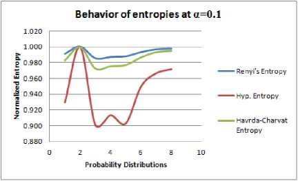
Fig. 1.

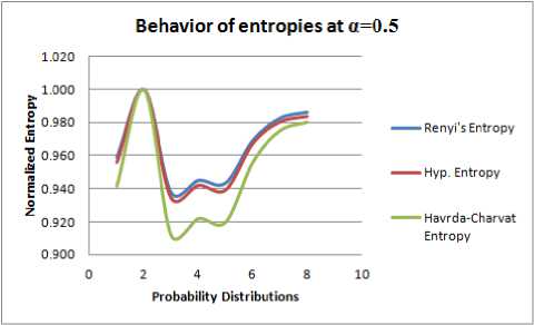
Fig. 3.

In Figure 1., the graph of the normalized values of three entropies under consideration for α=0.1 with respect to hypothetically chosen eight probability distributions is given.

Table 2-5 and Figure 2-5 have been constructed for similar purpose for α = 0.4. 0.5, 0.7, 0.75.

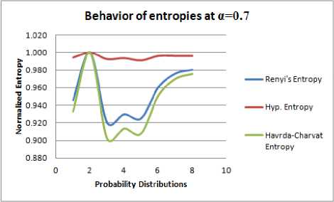
Fig. 4.

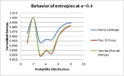
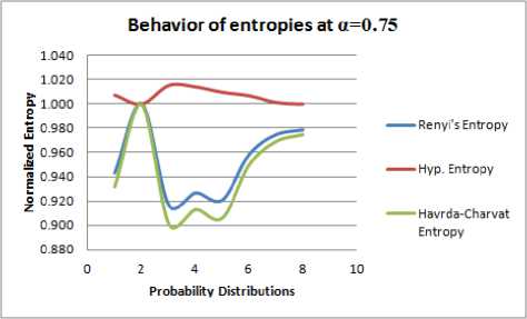
Fig. 5.

Fig. 2.

Based on the preceding comparisons the following observations can be made:

• 1.    The generalized entropies, with the Shannon Entropy as a special case, are almost consistent for different values of α, increasing α makes the measure’s values span a smaller interval. This means that as α increases, the measures become coarser and their discriminating power decreases. By changing value of α, Hyperbolic entropy can be made to oscillate on large interval or small interval. Further from the graphs in Figure 1-4, it can be seen that scalability of Hyperbolic entropy is much faster than Renyi and Havrda-Charvat Entropy.

• 2.    In Table 1-4, it is observed that maximum entropy corresponds to the probability distribution P ₂ for all the three entropies under consideration. But, from Table 5 it can be seen that Hyperbolic entropy is not in agreement with Renyi and Havrda-Charvat entropies in context of maximum entropy prescriptions of Jaynes[11]. That is, for a >  0.75, Hyperbolic entropy behaves differently. In other words, we can say that when extraneous factor α assumes value greater than equal to 0.75, we observe that the most unbiased probability distribution is not that what is expected from classical measures of entropy.

Further, using the probability distributions P ₁, P ₂,..., P ₈ , we construct Table 6 and Table 7 to show the superadditivity of Hyperbolic entropy.

From Table 6 and Table 7 it is concluded that:

Hhyp (P) + Hhyp (P) ^ Hhyp (P Pj),

J = 2,3,...,8                     .

Similarly, we can prove

H hyp ( P ) + H hyp ( P j ) ^ H hyp ( PP ), i , j = 1,2,3,...,8; i * j                     .

Therefore, hyperbolic entropy is super additive.

So, it can be applied to measure the information content of those systems which have several subsystems and total information provided by individual subsystems is less than that of information provided by whole system.

In biological studies it is observed that among the great amount of genes presented in microarray gene expression data, only a small fraction are effective for performing a certain diagnostic test. In this regard, mutual information has been shown to be successful for selecting a set of relevant and non redundant genes from microarray data. However, information theory offers many more measures such as the f-information measures which may be suitable for selection of genes from microarray gene expression data. Maji [12] tested performance of some f-information measures and compared with that of the mutual information based on the predictive accuracy of naive bayes classifier, K-nearest neighbour rule, and support vector machine and found that some f-information measures are shown to be effective for selecting relevant and non redundant genes from microarray data. In this type of study, the generalized information measure given in Eq.(7) proposed here may perform better, as it is more discriminative in comparison of some classical measures. Further, this measure seems to perform better in binary image segmentation.

• III. Applications of Generalized Hyperbolic Fuzzy Information Measure in Multiple Attribute Decision Making

A model to find the best alternative on the basis of multiple attributes is proposed here.

The model requires mainly the following:

• 1.    Available alternatives.

• 2.    Attributes.

• 3.    Weight of each attribute.

• 4.    Parameter α with which preference order of alternatives may vary.

Let X = { x 1 ,x₂,...,x n } be a finite set of alternatives and A = {a 1 ,a ₂,..., a m } be a finite set of attributes, and for      о <  a <  1,            w ^a = ( w a , w a ,..., w a )     ,

m w“ > 0, L w“ = 1 be the weight vector of the attributes i=1

a i ( i = 1,2,..., m ) which is not predefined.

Now, the model can be given in following three steps:

STEP 1 : Let R = ( p_A ( x i , a j )) _{n x m} be fuzzy decision matrix, where p_A ( x i , a j ) indicates the degree range that the alternative x satisfies the attribute a , the fuzzy entropy proposed by DeLuca and Termini[5] given in Eq. (4) takes the form ⁿ

^{H ( a} j ) = — 2i “ A ⁽ x i , ^a j ) ^log P a ⁽ x i , ^a j ) ⁿ

+ ⁽¹ - P a ⁽ x i , a j )) log⁽¹ - P a ⁽ x , -, a j )) ^}                 (8)

• , j = 1,2,.., m.

and the generalized hyperbolic measure of entropy given in Eq.(5) takes the form

H _a ( a j ) =--¹---

^J      sinh( a )

n

^ P a ⁽ x i , ^a j ) si^{nh( a} log P a ⁽ x i , ^a j ))

i = 1

n

• ¹    L (1 - P a ( x i ', a j )) sinh( a log(1 - P a ( x , , a j .)))    (9)

i = 1

j = 1,2,.., m .

STEP 2: The weight associated with attribute a is defined as follows:

H ( a )

Ot           a V J /       / •    1             \ wj = ^m---------, (j = 1,2,...,m.)

L H a ( a i )

i = 1

STEP 3: Finally, we construct a score function as follows:

m

S a ⁽ x i ) = У M a ⁽ x i , a j ) x w “ , i = 1,2,..., n j = 1

Alternative with highest score is the best choice.

Now, the above model is illustrated with the help of following example:

Example 3.1 Let us consider a customer who intends to buy a car. Five types of cars (alternatives) x i ( i = 1,2,3,4,5) are available. The customer takes into account four attributes to decide which car to buy:

• (1)    a ₁ : Price; (2) a ₂ : Comfort; (3) a ₃ : Design; and (4) a ₄ : Safety

Assume that the characteristics of the alternatives x i ( i = 1,2,3,4,5) are represented by fuzzy decision matrix

	R = ( M A ( x i	a j )) 5 x 4
Let	"0.7  0.5	0.6  0.6"
	0.7  0.5	0.7  0.4
	R = 0.6  0.5	0.5  0.6
	0.8  0.6	0.3  0.6
	0.6  0.4	0.7  0.5

We discuss the result for various values of a .

For a = 0 ; From fuzzy decision matrix we have

Table 8. Values of formula in Eq.(9) at α=0

H0(a1) H0(a2) H0(a3) H0(a4) 0.885282 0.98838 0.922965 0.97676 and Ун H o( ai) = 3.7733

i = 1

W = (W1 , W° , W0, Wj

= (0.2346, 0.2619, 0.2446,0.2589 )

By calculating we have

S ₀( x 1 ) = 0.59727, S ₀( x ₂) = 0.56995,

S ₀( x ₃) = 0.54935, S ₀( x ₄) = 0.57354, S ₀( x ₅) = 0.54619.

Based on the calculated values of Sa (xi) ,as above, we get the following orderings of ranks of the alternatives xi (i =1,2,3,4,5) ; x1 ▻ x4 ▻ x2 ▻ x3 ▻ x5.

Therefore the optimal alternative is x ₁ .

In the same manner we can find the ordering of ranks of the alternatives x ( i =1,2,3,4,5) for different values of α in Table 9.

Table 9. Values of S α (x i ) for α = 0.3, 0.5, 0.7, 0.9, 0.99

	α =0.3	α =0.5	α =0.7	α =0.8	α =0.9	α =0.99
S α (x 1 )	0.5975	0.5980	0.5988	0.5993	0.5987	0.6005
S α (x 2 )	0.5704	0.5714	0.5729	0.5738	0.5537	0.5759
S α (x 3 )	0.5494	0.5495	0.5497	0.5498	0.5489	0.5501
S α (x 4 )	0.5736	0.5739	0.5744	0.5747	0.5739	0.5755
S α (x 5 )	0.5465	0.5473	0.5484	0.5490	0.5487	0.5506

Again, based on results in Table 9, we get the following orderings of ranks of the alternatives x ( i =1,2,3,4,5) ;

For a = 0.3 x1 ▻ x4 ▻ x2 ▻ x3

For a = 0.5 x1 ▻ x4 ▻ x2 ▻ x3

For a = 0.7  x1 ▻ x4 ▻ x2 ▻ x3

For a = 0.8 x1 ▻ x4 ▻ x2 ▻ x3

For a = 0.9  x1 ▻ x4 ▻ x2 ▻ x3

For a = 0.99

,

From this discussion it is clear that x is most preferable alternative. But at a = 0.99 the ranks of preference of alternatives changes. Thus extraneous factor ‘α’ plays its role in order of preference and does not affect the choice of best alternative.

The proposed algorithm is also helpful in insurance sector (example 3.2), medical diagnosis (example 3.3), education (example 3.4) etc.

Example 3.2 Let us consider a customer who intends to get insured at an insurance company. Five insurance companies (alternatives) x_t ( i = 1,2,3,4,5) are available. The company takes into account four attributes to decide the suitability of customer for insurance:

• (1)    a ₁ : Smoking habit; (2) a ₂ : Cholesterol level; (3) a ₃ : Blood pressure; and (4) a ₄ : Adequate weight

Assume that the characteristics of the alternatives x i ( i = 1,2,3,4,5) are represented by fuzzy decision matrix

R = ⁽ M a ^{( x} i , ^a j )) 5 x 4

where m ( x _;, ^aj ) indicates the degree range that the alternative x_i satisfies the attribute a _{j .}

Proceeding with the data of example 3.1, it is concluded that company x is best choice to get insured.

Example 3.3 Let us consider a doctor intends to diagnose a patient based on some symptoms of a disease. Let five possible diseases (alternatives) say (x 1 :Viral fever, x 2 : Malaria, x 3 : Typhoid, x 4 : Stomach problem, x 5 : Chest problem) x i ( i = 1,2,3,4,5) have closely related symptoms or characteristics. The doctor takes into account four symptoms to decide the possibility of a particular disease:

• (1)    a ₁ : Temprature ; (2) a ₂ : Headache ; (3) a ₃ : Stomach pain ; and (4) a ₄ : Cough.

Assume that the characteristics of the alternatives x i ( i = 1,2,3,4,5) are represented by fuzzy decision matrix

R = (M A ⁽ xi , a j )) 5 x 4

where m a ( x i , a j ) indicates the degree range that the disease x_i satisfies the symptom a_j

Proceeding with the data of example 3.1, doctor concluded that patient is suffering from viral fever.

Example 3.4 Let us consider a person who intends to select a school for his ward’s admission. Five schools (alternatives) x i ( i = 1,2,3,4,5) are available. Man takes into account four attributes to decide the suitability of school for his ward: (1) a ₁ : Transportation facility; (2) a ₂ : Academic profile of teachers; (3) a ₃ : Past results of school; and (4) a ₄ : Discipline. Assume that the characteristics of the alternatives x_i ( i = 1,2,3,4,5) are represented by fuzzy decision matrix

R = (M A ⁽ xi , a j )) 5 x 4

where m a ( x i , a j ) indicates the degree range that the alternative x_i satisfies the attribute a_{j .}Proceeding with the data of example 3.1, father concludes that school x ₁ is best choice to secure admission for his ward.

It has been observed that the extraneous factor ‘α’ plays an important role in order of ranking of alternatives. So, two parametric generalized version of formula given in Eq.(9) may give better insight and flexibility in certain cases of multiple attribute decision making.

• IV. Concluding Remarks

A probablistic entropy measure can be additive, sub additive and super additive. In this paper, super additivity of generalized hyperbolic entropy measure (2) is tested with the help of hypothetical data. Therefore, one open problem, the application of super additive information measures is natural in this context. Secondly, we observed the fast scalability of generalized hyperbolic entropy measure (2) as compared to some classical generalized entropy measures [2,9] with respect to parameter a . This proposes another open problem: How this scalability is useful in various applications ? Sahoo et al.[13], Sahoo and Arora [14,15] applied one parameter entropy measures in image thresholding and analyzed the images on the basis of fact that how much information is lost due to thresholding. They observed that corresponding to the certain value of a the loss of information is least and produces best optimal threshold value. Thus, the parameter a in the generalized entropy measures is very important from application point of view. The entropy measure (2) may serve well in image thresholding problems in case of certain images.Two, three or four parameter entropy measures provide more flexibility of application.

A model for multiple attribute decision making(MADM) using generalized hyperbolic fuzzy entropy (5) is proposed here. The advantage of this method is that here we calculate the weight of an attribute from entropy formula itself whereas in the available methods of MADM weight of attributes is determined by experts. Moreover, fuzzy entropy has vital application in image processing problems [16,17]. Therefore, generalized hyperbolic fuzzy entropy (5) seems to be useful in image processing and pattern recognition problems.

Acknowledgments

We thanks the referees for their helpful comments for the improvement of the paper.