On the Performance of Classification Techniques with Pixel Removal Applied to Digit Recognition

Published Online August 2016 in MECS

• I.    I ntroduction

  Finding truly efficient methods of identifying and categorizing handwritten text is a decades-old problem that continues to plague researchers to this day [1]. In order to classify handwritten text a formal representation of each character (digit, symbol or letter) must first be established. In the early stages of classification developers sought to determine patterns based on the dimensions of each character, measuring them with rulers and compasses. They saw that there were several physical characteristics that determine patterns in the development of handwritten information [2] [3] [4]. In 1954 T. L. Smith alluded to six defining characteristics of

handwritten text. These include: pressure; form; spacing; speed; size; and slant [3]. Since then, there were many researchers that have added to this set of criteria that defined the characteristics of each handwritten character.

Texts that were classified using these simple yet tedious characteristics limited the development of more dynamic methods of statistical classification for handwritten figures. It was not until the success of the German Bundeskriminalamt (the Federal Criminal Police Office) with the development of the computerized image processing and pattern recognition system, FISH (Forensic Information System of Handwriting), in the early 1980s, that the rest of the world took notice and developed their own systems for computerized numerical imaging. FISH enabled countries to have interactive work with the document examiner, to enable retrieval of the closest match from a large database of handwritten digits and letters [5]. It has formed the framework for many other databases worldwide including those used by the United Kingdom and the United States of America [2].

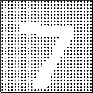
Fig.1. A Block Identifying the Outermost Pixels of an Example of the Digit “7”

This study focuses on one such database in particular, the MNIST (Mixed National Institute of Standards and Technology) database which is a modified version of the NIST (National Institute of Standards and Technology) dataset. The MNIST database is a large set of handwritten digits (0 through 9) which consist of 60, 000

training data points and 10, 000 testing data points. Each observation is a 28 × 28 block of pixel variables as depicted in Fig. 1. Pixels are the individual values that make up each block. Each pixel in the MNIST has a single pixel value ranging from 0 to 255. These 256 values represent the different grey intensities and are very common in the quantization of images [6]. The darker pixel the higher the pixel value would be.

This change in format of defining characteristics of digits does not equate to any loss in the physiognomies that comprise each character as described by T. Smith [3] and Livingston [2]. There is a battery of transformations that can be used on such databases to extract and exploit of its linearity and curvature handwritten text. The Hugh Transformation was used on the MNIST databases to characterize digits within defining physical properties including holes, right-entries, left-entries, cross in the centre, extremes, horizontal and vertical intersections, and distance [7]. Kumar et al. [1] used mathematical morphology to exploit the shape of the ten digits found MNIST in the database. Morphology was used to separate digits into two groups: (a) Groups with blobs (or holes) {0, 4, 6, 8, 9}; and (b) Groups with stems {1, 2, 3, 5, 7}. Jankowski and Grabczewski [8] also played with the shades of data points through a special type of normalization called darkening.

From the above studies there seem to be no loss of information due to the digital format of MNIST dataset as displayed visually by Fig. 1 but are all the pixel values necessary for the classification of handwritten digits? This study seeks to question the need for and the use of the outermost pixels that define each data point of MNIST database, by comparing the impact, on time and accuracy, of its removal on four classification techniques. The term “white noise” will be used as a benchmark in determining the impact on accuracy of the classifier. White noise suggests a time series that does not contain any information that would help in the estimation process (these variables have zero mean and constant variance). It is the residuals of the true model that captures the data fully [9]. The study proposes that the outermost pixels (variables) of the blocks, which represent each digit, should have a negligible impact on the ability of a classifier to correctly identify the class of a digit. This is because the outermost pixels contain little information about each digit as displayed in Fig. 1. As successive groups of the outer variables are removed, the expected impact on classification should become more noticeable, as greater amounts of defining pixels are lost. Hence, these outer variables will be seen as the producers of noise and the effect on the accuracy of classification will determine the level of noise. There can be three possible impacts:

• i.    A negative noisy effect, when accuracy falls.

• ii.    The white noise effect when there is zero impact on accuracy and results.

• iii.    A positive noisy impact when accuracy increases.

Thus the aim will be to determine exactly how these outer variables impact the level of noise and the time each takes to classify each observation of the MNIST dataset for four classification methods. The chosen methods are:

• •    The Recursive Partitioning and Classification Trees (RPCT)

• •    The Naive Bayes (NB) Classifier

• •    The k- Nearest Neighbour (k-NN) model

• •    The Support Vector Machine (SVM) model

• II.    T he C lassifiers

The classifiers discussed have performed well under different situations. We now discuss each of the four methods we compared.

• A.    RPCT Method

The RPCT [10] algorithm is a nonparametric, supervised learning statistical method of classification. It tends to ask a series of binary questions. It starts at a unique point called a root node which considers the entire training dataset. This dataset is then broken down into two daughter nodes that are subsets or partitions of the dataset. Each node has a binary split of classifiers which are variables that determine the level or response. The split is determined by Boolean conditions (that is, “yes” if satisfied and “no” otherwise). Any node that does not split is a terminal node which gives a class, if the node does not terminate it is called a non-terminal node which can be further split.

However, in cases where there are large numbers of input variables, as with the MNIST dataset, where data points are defined by 784 input variables or pixels, a tree can be outrageously large. With categorical variables, there can be a possible 2  -2 splits (where n is the number of categories). Although many of these splits are said to be redundant, the number of node splits will be tremendous and saturated trees may be enormous [10]. Very large trees may complicate the classification process and delay calculations for decisions on predictions. Large trees can also lead to the problem of over fitting the model and misclassification.

To repair the problem of overfitting, earlier growers thought the solution would be to restrict growth by placing conditions on the nodes, as to where they were terminated. This was deemed to be a flawed practice, trees were to be grown to saturation then pruned (the strategic removal of branches of trees) using simple statistical techniques to reduce tree size. Branches are pruned based on a computed misclassification rate for each node [11]

An effective estimate for the misclassification rate is the Redistribution Estimation Misclassification rate is given by R (τ) of an observation in the node τ [10].

r(τ)= 1-max к Р ( к |τ),              (1)

where k describes a particular class or level

Let T be the set of tree classifiers and T̆ = {τ1, τ2, τ3, ......... τn} denote the set of all terminating nodes of T, the estimation for the misclassification rate is

R (T) = ∑ ∈ ̆ R (τ)Ρ(τ) =∑S = 1 R(τ)Ρ(τ)    (2)

for T where P(τ) is the probability that an observation falls into node τ .

If P( τ ) is estimated by proportion p( τ ) of all observations that fall into node τ , then the redistribution of R(T) is:

Rre(T) = ∑S=1r(τ )р(τ )=∑S=1 R re (τ ),    (3)

where

R re(τ )=r(τ )р(τ).              (4)

Once R(τ) is estimated for each node τ ∈ T_max , pruning takes place from the most recent splits (bottom of the tree) up to the root node, until the tree reaches its ideal size. The split choices at the lower portion of the tree do often become statistically unreliable [12]. A pruned tree is a sub tree is of the larger tree and since there are many ways to prune a tree we choose to remove the sub trees which maximize misclassification rate [11]

• B.    NB Method

The NB classifier is a probabilistic method of classification that is deemed to be both simple and powerful. It is based on the naive assumption that there is independence between each class and all of its classifying variables. It also assumes that classes are engendered form a parametric model, as such, the training data is used to compute Bayes–Optimal Estimates for the model parameters. It then classifies the data for testing by applying Bayes rule to use the generative model in reverse. That is, calculating the subsequent probability that, a class could generate the questioned test data point. Thus classification becomes the simple issue of choosing the most probable class for the given test data points [13] [14].

The NB theory assumes that classes are identified using a mixture model parameterized by 0. The mixture model consists of a combination of components cj ∈ C = {c1, c2, c3,.......,cs}. Each data point y is created by firstly selecting components using priors, P (cj| 0), and secondly, having these mixture components generate a class or digit according to its own parameters, with distribution P Ы0).

The Bayes theorem states:

P(y|Ɵ) = P(y|c i ,c2,.......,c)= - ⁽ ) ( ^, ^ , , | ^У- ⁾ , (5)

(^L1^{, l}2 ,, , ^LS)

where 0 can be a combination of any or all of the components c i

Using the NB’s naive assumption of independence

P(ci|y,ci,c2,.......,c)= P(ci |y),

Therefore,

P(y| Cl, C2,.......,c s ) = 5 ( ()∏, ,  .(. | ) ,(7)

(L1,12 ,,

Since P(Ci , C2,.......,cs) is a constant, given the input, the value which the P(y| Ci , C2,.......,cs) is given by

P(y)∏i=l Р(сi|y),

Thus the estimate for y,

̂= argmaXy P(y)∏i=i Р(сi|y).       (8)

Now, P(y) is simply given by the relative frequency of y, thus the probability that maximizes the estimates of y is really given by P (c i |y) [15].

To give an understanding of how this may be done, two methods are briefly outlined. The first being a classical method and the second is more modern approach to calculation.

• (i)    The multivariate Bernoulli NB

• (ii)    The Gaussian NB

(i)The multivariate Bernoulli NB [16] for generation, base each class on a number of independent Bernoulli trials where each 0 in an observation, y, is asked whether or not an attribute c i occurs for each data point (0 for no and 1 for yes). This is done for each attribute and probabilities are calculated given multiple Bernoulli trials.

P (c i |y) = P ( i | У ) Ci +(1- p ( i | У ))(1- Ci ),       (9)

where p ( i | У ) is given by the number of times c i appears in the total components of y.

• (ii)    The Gaussian NB uses the Gaussian classifier algorithm. The likelihood of each class is given by

p (=. | d )= =^= exp (- ⁽ щ ⁾ ),       (10)

√ 2na^ \         )

where Цд and a^ are the estimated parameters using the maximum likelihood of class d.

The Gaussian NB is a very popular measure and is used as the basis for many statistical programs today inclusive “naiveBayes” operator in the R statistical software [16], which was used in the formulation of the model for this paper.

• C.    k-NN Classifier

The Nearest Neighbour (NN) classification method is an example of one of the more archetypal and widely used, discriminate training methods for classification. It is a form of unsupervised machine learning algorithm that is often referred to as lazy, as it waits until asked, to classify variables. This process bypasses probability estimation and uses the entire sample set to estimate posterior probabilities, classification can be made using these properties given by metric distances. The NN model assumes that data of the same category generally exist within close proximity in a feature space and share similar properties. Hence properties are obtained by a nearby sample, by applying this to pattern recognition. The test set categories can be inherited from the category of its nearest neighbour in the training dataset.

Consider the training sample {y1, y2,...............,yn} of m categories {c1, c2,............, cm}. Each sample of yj is labelled with a corresponding category ci. The distance function given by dis(a, b), is a non- negative real value function for all pairs of yi of the training set. It is regarded as the nearest neighbour of the y of test set if dis(y, yi) < dis(y, yj) for all i^j. Thus any y of the test set would have the same class as yi of the training set [17].

The k-NN model uses this principle when taking into consideration the k closest neighbour samples in proximity of y, as specified by the k samples used of the same specific category. The value of the k is a smoothing parameter of decision boundaries and is empirically determined. In the case of a tie, the k-NN model simply re-votes or decreases the value if k by one [13] [14]. The k-NN model boils down to the simple NN model when k=1.

There are several advantages [17] to using the k-NN model of classification. They include:

• (i)    No training process is needed for data, to classify the unseen samples.

• (ii)    The k-NN model is very effective when using both small and large datasets.

• (iii)    New training samples can easily be added during run time.

• (iv)    The k-NN method achieves the optimal error rate generated by Bayes classifier when both the number of training data and the value of k increases, and k/N tend to zero.

The inherent problem with the k-NN classifier however, is that it requires very large quantities of storage space to run the model. There are two methods that seek to deal with this issue of improving storage or the RAM required for modelling. The prototype-selecting and the prototype-generating approaches are used to [17]. Prototype-selecting method uses a subset of the training dataset, chosen with some experimental method (trial and error) to maintain the system’s performance. The prototype generating system however, depends upon a clustering algorithm that condenses the data, using distortion methods, to give fewer representatives for each class.

• D.    SVM Method

A SVM [10] is an example of a supervised machine learning technique of classification. The SVM algorithm seeks to classify data points by creating separations between different classes identified in the model. The support vector mechanism is a type of supervised machine learning that can be both linear and non-linear. It involves optimization of the convex loss function under a set of constraints, unaffected by minima. It seeks to divide classes using hyperplanes that maximize the distances (separations) between classes.

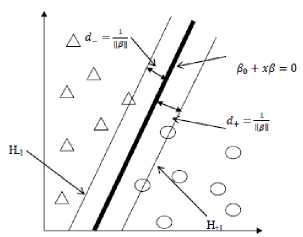
Fig.2. The Linearly Separable Instance of the SVM

Separating hyperplanes divide data into two classes without error as shown in Fig. 2. There can be an infinite number of them for any one dataset. The task is then to determine the optimal hyperplane, that is, the one which maximizes the separation (distance or space) between classes which can be easily done in the linear case.

However the use of nonlinear transformations is problematic since it involves the computation of inner products in a high dimensional space M.

The use of the kernel trick, first implemented by Cortes and Vapnik [10], helps to de-complicate this problem. The idea is opposed to calculating the inner products in M, where it is computationally expensive to derive, use a nonlinear kernel function,

К (х^х , ) = (ФО^Ф^к      (11)

in a separate input space, which speeds up the computations. A linear SVM is then calculated in a different sample space.

A kernel is a function, К : ^^r x ^^r ^ ^ , for all X ,y E ^²,

К (х,у) = (Ф(х),Ф(у)).               (12)

The kernel function was devised for the computation of the inner products in M by using input data. Hence the inner product (Ф(х), Ф(у)) is substituted into the kernel function. All that is required of a kernel function is that it needs to be symmetric, that is

К (х, у) = К(у, х), and it satisfies the inequality

[ К(х,у)]2 <К(х,х)К(у, у),(14)

derived from Cauchy- Schwarz inequality.

The kernel functions can take several forms including:

• i.    The Gaussian Radial Basis Function

К (х,у) =ехр{-Ы2}

• ii.    The Laplacian function

К ( х , У )= exр{- ^{‖   ‖} },           (16)

• iii.    The Polynomial of degree d Function:

К ( х , У )= 〈 ( х , У ) с 〉 ^й             (17)

where c ≥ 0 and d is an integer.

The polynomial of degree d function is commonly used in handwritten digit classification and is the function used in this paper.

In Multiclass cases, where training data is represents n >2 classes, SVM may train data for classification in two ways:

• i.  The one-versus-rest method

• ii.    The one-versus-one method

Each classifies multiclass training datasets using multiple binary techniques. The one-versus-rest finds separations between each specific class and all the remaining classes. Whilst one-versus-one pins each class against another class, resulting in () comparisons.

The one-versus-rest classification method’s success depends on the number of classes and whether one category outweighs the other categories in deciding the most probable classification for each test data point. On the other hand, the one-versus-one approach suffers from having to use smaller subsets for training classifiers which may increase variability. Either way they both give more than acceptable results when carrying out classification.

Each colour represents a different frame. There the first ten frames are identified out of a total of fourteen possible frames. These variables were trimmed original MNIST database and the findings are based on the successive trimming of these ten frames.

In Fig. 3 the yellow frame represents the first frame. Trimming these pixels turns each data point in the dataset to a 26 × 26 row of pixels, which would comprise the trim 1 dataset. Similarly, the first two frames (yellow and red) were removed from each data point to give the second trim, the trim 2 database formulated from the corresponding 24 × 24 pixel matrix. This was repeated another eight times until the tenth and final trim, data points derived with a 08×08 pixel matrix. The trimming process therefore creates eleven variations on the MNIST dataset.

Each time a frame is removed the total number of pixels is also reduced by

10² + 8(2-x), X =1……10, (18)

where X is the number of trimmed frames. This in turn can be summed to give the total number of pixels lost from the original MNIST database, given by

116n-8∑Г=1 xi, i=1,2,…10. (19)

The objective is to measure the effect of the removal of the pixel values, as determined by change in accuracy rate and modelling time, on each classifier.

The Visual Impact, of Trimming, on the Images of Each Digit

The following images show the visual impact of the ten successive trims on the MNIST dataset. The training set depicted on the left and the testing set on the right.

III. D ata T rimming

Trimming is as the process of removing the outer most pixel values of each observation. The number of pixels is a fundamental consideration in any image/pattern recognition method.

о    /а

3    45

6     7?

6    7    8    9   10   11   12   13   14   15   16   17   18   19   20   21   22   23   24   25

58   59   60   61   62   63   64   65   66   67   68   69   70   71   72   73   74   75   76   77   78   79   80   81

87   88   89   90   91   92   93   94   95   96   97   98   99  100  101  102  103  104  105  106  107  108

116  117  118  119  120  121  122  123  124  125  126  127  128  129  130  131  132  133  134  135

146  147  148  149  150  151  152  153  154  155  156  157  158  159  160  161

175  176  177  178  179  180  181  182  183  184  185  186  187  188

203 204 205 206 207 208 209 210 211  212 213 214 215

232 233 234 235 236 237 238 239 240 241 242

514 515

261 262

518 519 520

541 542 543 544 545 546 547 548 549 550

567 568 569 570 571 572 573  574 575 576 577 578 579

595 596 597 598 599 600 601  602 603 604 605 606 607 608

622 623 624 625 626 627 628 629 630 631  632 633 634 635 636 637

648 649 650 651  652 653 654 655 656 657 658 659 660 661 662 663 664 665 666 667

675 676 677 678 679 680 681 682 683 684 685 686 687 688 689 690 691 692 693  694 695 696

702 703 704 705 706 707 708 709 710 711 712 713  714 715 716 717 718 719 720 721  722 723 724 725

756 757 758 759 760 761  762 763 764 765 766 767 768 769 770 771  772 773 774 775 776 777 778 779 780 781

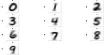
Fig.4. The Blurred Examples of Digits 0 through 9 from the Original MNIST Database

О   J^

3     45

Ь     7

q

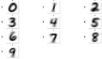
Fig.5. The Blurred Images of Digits 0-9 after the First Trim

Fig.3. The Ten Different Frames of Pixels That Represent Each Data Trim

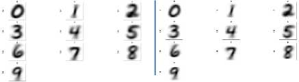
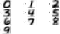
Fig.6. The Blurred Images of Digits 0-9 after the Second Consecutive Trim

These outer pixels are broken up into frames as is depicted in Fig. 3 by the coloured rectangular blocks.

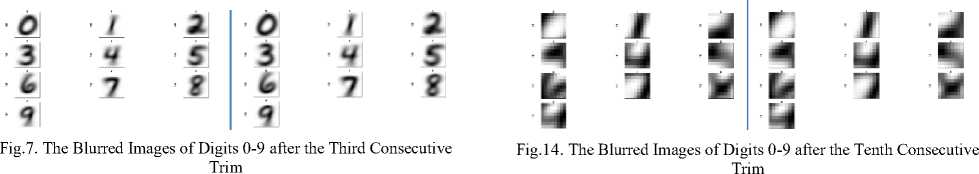
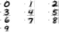
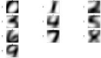
Fig.8. The Blurred Images of Digits 0-9 after the Fourth Consecutive Trim

IV. M ethodology

To carry out this investigation two steps were used. Subsequently, each was individually timed to determine the impact of frame removal on the efficiency of the classifiers. The steps are outlined in the following:

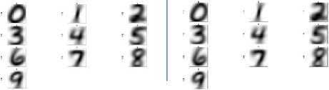
Fig.9. The Blurred Images of Digits 0-9 after the Fifth Consecutive Trim

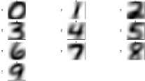
Fig.10. The Blurred Images of Digits 0-9 after the Sixth Consecutive Trim

• a)    (a)The training (modelling) of data. This was done using a training set of observation points where the observation classes are already known. Allowing programs to identify the criteria and formulae (depending on the model) to classify each data point into a class.

• b)    The testing of model (classification). This was done using the model, derived in (1), to classify a different set of data points (test dataset). Models use the variables of the associated test dataset to predict the class of each data point blindly¹. Its strength or quality is then measured using the accuracy rates, which are calculated by comparing the predicted classes with the actual classes of the test dataset.

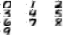
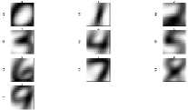
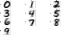
Fig.12. The Blurred Images of Digits 0-9 after the Eighth Consecutive Trim

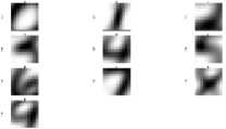
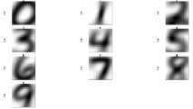
Fig.11. The Blurred Images of Digits 0-9 after the Seventh Consecutive Trim

Predicted Class

Actual Class			2		-	7	7		7	9
0	1138	2	1	3	0	1	71	0	27	20
1	0	1357	L	5	0	1	12	0	26	8
2	137	41	141	215	1	6	387	3	279	16
3	74	87	4	607	0	2	98	8	294	143
4	31	16	3	14	103	5	181	8	173	650
5	152	49	4	37	1	35	111	0	608	138
6	11	16	4	1	0	0	1173	2	18	2
7	12	8	1	17	2	0	8	393	48	843
8	20	204		10	1	2	55	1	681	261
9	9	20	0	4	4	1	6	9	38	1181

Fig.15. An Example of a Confusion Matrix

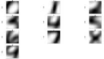
Fig.13. The Blurred Images of Digits 0-9 after the Ninth Consecutive Trim

The result for each prediction was visualized using a confusion matrix as depicted in Fig. 15. The diagonal elements represent where the actual and predicted classifications intersect. These are the correct classifications. The other off-diagonal elements, of the matrix are the misclassifications for each data point. The confusion matrix also provided the added knowledge of what predictions were made. Comparisons could then be made between trims for each model.

The confusion matrices was used as a tool to tell whether or not the models (of the same classification method) give the similar results, since accuracy rates alone cannot sufficiently determine the presence of white noise . To do this, both the accuracy rates and the

classifications (the off diagonal and diagonal elements of the confusion matrix) must be consistent.

The software used for this project was R and in R the models are built on five–fold internal cross validations of the training database. This is where the dataset is broken into five equal subgroups and modelled using the defined parameter. The results are then aggregated to give the optimal model. This process is done the same way each time thus producing identical results for identical datasets each time the model is ran. This heterogeneity of the different implemented classification algorithms is usually seen as a problem with the R programming language. However it works as an advantage, as conditions for modelling and resampling for cross validation remain constant. Heterogeneity, in modelling, in this instance, was very important as it was the data that is the controlled variable and not the classifier. Changes in accuracy rates should reflect the variations in number of variables due to trimming and not differences in the resampling methods.

• V.    R esults

In the RPCT method, the first four models representing the original dataset (no trim) and the first three trims, Table 1 shows, that they produced the identical result of an accuracy rate of 61.96%. The confusion matrices representing the no trim to trim 3 models also produced identical classifications for each. This exemplifies the presence of white noise variables, in that, with the removal of these, results in identical accuracy rates and classifications.

In the fourth trim the accuracy level slightly dipped to 61.84% but then continued to increase to its optimal accuracy of 63.34% in the sixth and seventh trims. It can again be appreciated that, where the two accuracies were identical that their respective confusion matrices produced identical results. From the eighth trim to the tenth trim results waned, with its lowest value of 54.18% accuracy rate on the tenth trim.

Table 1 shows the results obtained from the SVM model of classification which shows that without any trimming the model gave a 97.91% accuracy rate. It fell slightly by 0.01% on the first trim then rose to 97.95% on the second trim. This trim was the strongest results. The accuracy slightly decreased to match the initial results of 97.91% in the third and fourth which increased by 0.01%. From this point the results in the decline in small increments, it was only in the eighth trim that the accuracy level was below 95%. The classifier, however, was unable to model the data on the tenth trim.

Table 2 shows the time the RPCT model took to train each dataset, it was found that it decreased steadily from the no trim to the trim 10 model. The reduction of variables represented by the removal of frames aided in the improvement in the speed of modelling regression trees. The prediction times were almost instantaneous for the regression trees for each of the eleven models.

Table 1. The Accuracy Rates (%) For Each Classification Method

Model	RPCT	NB	k-NN	SVM
No trim	61.96	53.52	96.91	97.91
Trim 1	61.96	52.18	96.91	97.9
Trim 2	61.96	53.64	96.91	97.95
Trim 3	61.96	62.34	96.87	97.91
Trim 4	61.84	74.0	96.8	97.92
Trim 5	63.2	79.47	96.84	97.88
Trim 6	63.34	81.05	96.59	97.74
Trim 7	63.34	78.98	95.63	97.11
Trim 8	60.94	78.98	93.23	95.41
Trim 9	58.72	72.11	88.6	91.73
Trim 10	54.81	63.08	79.81	NR

Table 2. The Times (seconds) for Modelling (M) and Classification (C) for each Method

Model	RPCT		NB		k-NN		SVM
	M	C	M	C	M	C	M	C
No trim	105		6.7	172	8184.	1799	2666	200
Trim 1	98		6.5	151	6918	1543	3899	111
Trim 2	82		6.5	191	5571	1343	2873	195
Trim 3	71		8.7	143	4209	1013	2753	108
Trim 4	60		8.9	156	3602	975	2315	68
Trim 5	49		9.0	120	2296	608	2214	87
Trim 6	39		8.6	113	1855	462	1987	179
Trim 7	31		7.9	111	1713	450	1849	116
Trim 8	23		8.2	88.	1117	242	1830	74
Trim 9	16		8.2	84	753	163	1955	74
Trim 10	10	_	7.2	82	506	105	NR	NR

The NB classifier, without trimming, had an accuracy rate of 53.52%, which dropped by more than a percentage point after the first trim to 52.18%. However, from the second trim upward to the sixth trim the accuracy levels steadily increased reaching its optimal accuracy rate of 81.54%. The seventh and eighth trims, gave the same accuracy rate of 78.98%. The ninth trim saw a more than 6% drop in accuracy to 72.11% and then the tenth dipped by a 9% to 63.08% which is still an almost 10% improvement on the 53.52% accuracy rate obtained in the no trim model.

The confusion matrices for each of the models were very different in terms of accurate accounts of digits. For example the confusion matrices representing classification of digit without trimming (no trim) and the model representing one trim (trim 1) of the data, arguably the two models with the two most similar datasets, gave rise to very different predictions. Even on the seventh and eighth trims, where the accuracy rates were the same, the confusion matrices were very dissimilar.

The time taken to formulate the NB models as seen in Table 2, fluctuated although it was quite small as compared to the time needed for classification. The time necessary for predictions for each trimmed model whilst it had slight fluctuations, there was an overall decrease in this time from the original set. The NB model was not, in general, a time consuming classification model as compared to the other models.

The k-NN method gave the same results as that of the no trim model for the first two trims with an accuracy rate of 96.91%. However it steadily declines from the third trim model onwards. The accuracy level remained above 96% up to the sixth trim model, from the seventh trim model onwards level of inaccuracy increased at an increasing rate with an almost 5% decrease between the eighth and ninth trim model and a 9% change between the ninth and the tenth trim models to give a 79.81% accuracy rate.

The k-NN model shows that results for the first six trims were comparable, with the first three models, where the accuracy levels were identical, having confusion matrices that were also identical. The confusion matrices for the last four trims were very different since accuracy rates decreased substantially.

Table 2 shows that the time it took for both model building and prediction decreased as the number of trims increased. The difference between the no trim and first two trims is over 2600 seconds and greater than 400 seconds, respectively, which is a vast improvement. The time taken to produce models and classify observations is a flaw that is intrinsic with the k-NN classifier; as such decreases in time due to the removal of frames can be very helpful towards dealing with this issue.

The confusion matrices showed that the predictions made were very similar though not identical for the first six trims. The no trim model and the trim 3 model, though they have of same accuracy rate, the actual predictions were not identical.

The time for modelling and classifying the data with respect to each trim varied as compared to the other three models which generally decreased over the trimming process. However, the times for prediction SVM algorithm, for all the subsequent models were less than that of the no trim model.

• VI.    D iscussion

Given that after the first three consecutive trims the accuracy rate of 61.96% (Table 1) remained the same and identical predictions are given in their respective confusion matrices as compared to the no rim model, for the RPCT method of classification, shows that the model did not need the variables in the first three frames to produce result identical to that of the original MNIST dataset. It can be inferred that the first three frames of variables were white noise variables. However, the no trim model, did not give the best results, as this was not the best utilization of variables given. The optimal results were achieved at the seventh trim where its accuracy was 63.34% with a reported time of just over 31seconds, shown in Table 1 and Table 2 respectively. This demonstrated that more centralized datasets with less variables produced better results as the models were better able to utilize its variables to this point.

The RPCT model had very small changes in accuracy rates over the first seven trims, which reflects its stability as a classifier [18] [19]. From the eighth trim onwards, however, it had a negative noisy impact with sharp declines in accuracy.

The NB classifier on the other hand gave the weakest results in handwritten digit recognition using the MNIST dataset [8] [18]. Although many studies were devoted to finding ways to improve the NB classifier [20] it still seems to fall behind the other three statistical classifiers in the prediction of handwritten text. This was confirmed when NB had the worst initial results with the original (no trim) MNIST dataset giving a low 53.52% accuracy rate. However this quickly changed from the third trim (trim 3), where there was a positive noisy impact. Results increased until there was a substantial raise of over 27% on the initial no trim model, to 81.54%, in trim 7. Thus the trimming had an encouraging impact since it improved the result obtained by the NB classifier. However, in instances where accuracy rates were similar or even identical the set of predictions were very different. This may be due to the fact with each trim of the data the NB classifier chooses a different set of priors for each mixture components model. Smaller numbers of variables seem to have positive effects on the NB classifier.

Giuliodori et al. [7] used several features to transform the MNIST dataset into a thirteen variable dataset and found great improvement in the results obtained. Palacios-Alonso, Brizuela and Sucar [21], found that the NB classifier performs worse when relevant explanatory variables are reliant on irrelevant ones, such as the zeros in our dataset. Thus with each trim the NB model is better able to utilize the given explanatory variables. The removal of frames of pixel values did not prove the existence of white noise in this instance, but, it proved to be quite promising. The accuracy rates increased steadily showing the positive noisy effect of trimming on accuracy rates in the NB classifier.

The k-NN model seemed to stay truest to the classifications made having very similar results between trims even though it did not respond well to the varying datasets from studies by Bennett and Campbell [14] and Oxhammar [19]. The no trim model had an accuracy rate of 96.91% and identical results were produced for the first two trims. Consequently this was the best result obtained by the k-NN classification model. This showed that the k-NN model did not necessarily need the first two frames of pixels to produce the corresponding results to the original MNIST dataset. Thus the variables found in the first two trims are not necessary for the classification of variables. This leads to the belief that the first two frames of pixels are white noise variables. The k-NN modes are relatively quiet up until the sixth trim, after which, had a negative noisy impact as accuracy fell more considerably.

The removal of the first two frames of data reduced the time to predict digit over 2600 seconds to model and over 400 seconds for predicting. The k-NN model suffers from being expensive with respect to storage [17] which tends to have an adverse effect on time. Fig. 18 shows that of all the four models, the k-NN model is the most expensive with respect to time, removing these unnecessary frames helped with combating this issue.

Compared to the other three models the SVM gave the strongest results [14] [19] as shown in Fig. 17. The accuracies in the first six models slightly fluctuated around 97.9%. The SVM model level of accuracy never fell below 91% although it was the only classification method that could not produce results for the tenth trim, ceteris paribus , as the other ten SVM models. The confusion matrices produced showed that results show noticeable differences in classification of digits. With only minor changes to accuracy levels for the first seven trims and in the remaining trims not dipping below 91% accuracy rate, the SVM model can be seen as relatively quiet over the trimming process with the lowest standard deviation rate of 1.995% (Table 3).

The SVM model was the second to the k-NN model in time consumption. With the removal of each frame the modelling time for the SVM decreased steadily in eight out of the ten models and there was an overall decrease in classification time. The removal of frames helps the SVM model to improve on what is generally a more time consuming classifier.

Fig. 16 gives a synopsis of the accuracy trends for each of the classifiers. It shows that, trim for trim, the SVM model performs the best of all the four methods; the k-NN is second best and the NB and RPCT rounded off the bottom.

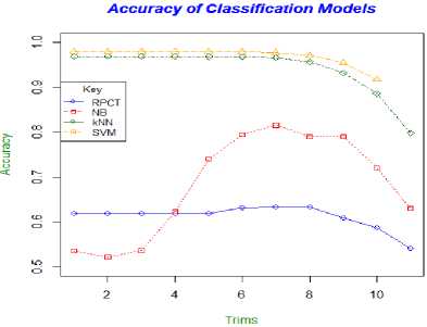
Fig.16. The Accuracy Trend Lines for Each Classification Model

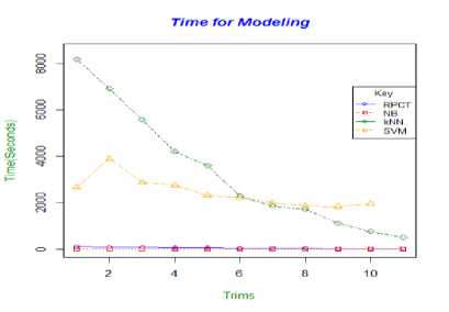
Fig.17. The Time for Modelling for Each Classification Model

As the trims of data increase the centre of each data point is magnified, from a visual stand point, all digits could be easily recognized up to the seventh trim, and real loss of visual perspective only comes at the ninth and tenth trims (Fig 4 - 14). All four of the classification methods seemed to have reflected this descent with results by plummeting at the seventh or eighth trim as depicted in Fig. 17.

Table 3. The Mean and Standard Deviations of Each Classifier

RPCT   NB    k-NNSVM

Mean (%)       61.22    68.17     94.196.95

Std Dev (%)      02.67       11.53     05.381.995

The overall trends in accuracy levels look very similar for the RPCT, k-NN and SVM models, however the changes in the number of variables, by removing frames, have the greatest impact on the NB model. This is reflected in the high standard deviation rate of 11.53% of the NB model as compared to the 2.67%, 5.3% and 1.995% of the RPCT, k-NN and SVM models respectively, as depicted in Table 3. Although the NB classification model had the worst initial results of the four, it ended with the third best overall performance.

Time for Classification

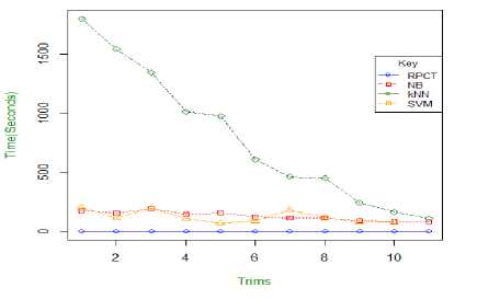
Fig.18. Modelling and Classification Time Trend Lines for Each Classification Model

Fig. 18 gave prospective to the general trends in both modelling and classifications times per algorithm over the eleven models. In both cases the k-NN classifier was the greatest consumer of time initially however with the successive removal of frames, for both modelling and classifying, its times became comparable with the other algorithms. The RPCT model had quite low and stable times however, the NB and SVM times fluctuated during the entire process, the SVM showed the greater variation of the two. With respect to modelling, however, the SVM times were exponentially larger than the NB method. This showed some difficulty by the classifier in modelling as frames were removed from the original MNIST dataset. This was confirmed as it was the only model unable to produce results from the tenth trim dataset.

• VII.    C onclusion

Each model was affected positively by the trimming of the MNIST dataset. With the exception of the k-NN algorithm, the classification models were able to see improvements in their accuracy rates. The greatest benefits were seen by the NB model whilst the other two enjoyed moderate improvements. Although the k-NN model had no improvements with regards to accuracy, the true benefit was in the reduction of storage space needed for the modelling and classifying of data. This lead to a reduction in the time needed to for processing, which is pivotal for a very time consuming algorithm. Both the RPCT and the k-NN methods showed signs of the presence of white noise but it was the k-NN model that really exemplified this effect.

Based on the positive results attained from removal of the outer most pixels, although, not producing the ideal white noise effect for each method it can be determined that it would be beneficial to trim some frames from the MNIST database. Exactly how many frames of pixels to be trimmed depend on the method of classification that is used. If it were to be based on the combined results obtained from each model, it could be recommended that the removal of at least two frames of pixels would be beneficial to the modelling process.

• VIII.    R ecommendation

It is recommended that when modeling using the MNIST dataset without transformation that the trimming process be used for possible enhancements in results and for possible reductions in classification times.