On the stability of two-dimensional flows close to the shear

Mathematical models that describe two-dimensional or spatially periodic fluid flows are widely used to study various natural phenomena in the atmosphere and the ocean [1]. In [2], a model of two-dimensional creeping motion of viscous liquid in a flat channel is considered. Based on a priori estimates, the solution of the problem is constructed and its properties are investigated. The Kolmogorov problem for a two-dimensional viscous fluid under the influence of spatially periodic external forces is considered in [3]. Using the Galerkin method, stationary and spatially periodic solutions are found numerically. In [4] nonstationary time-periodic structures are obtained using long-wave perturbations of the Kolmogorov flow.

In this paper we consider the two-dimensional ( x = (x1,x ₂ ) G R ² ) viscous incompressible flow driven by an external forces field F ( x ,t) that is periodic in x1 and x ₂ with periods ℓ1 and ℓ2 , respectively. The flow is described by the Navier–Stokes equations

∂v д^- + (v, V)v — vAv = —Vp + F(x, t), div v = 0, where v = 1/Re is the kinematic viscosity and Re is the Reynolds number. The period 11 = 2n, and the ratio of the periods is characterized by the wave number a: 12 = 2n/a, a ^ 0. Let (f) denote the average with respect to x1, ((f)) denote the average over the period rectangle Q = [0,11] x [0,l2]:

ℓ 1

^(f ) = T / f^(x,t) dx i , ℓ1

(( f )) (t) =

и / f

Ω

dx ₁ dx ₂ .

The spatial average velocity is assumed to be given: (( v )) = q . The velocity field is assumed to be periodic in x1 , x2 with the same periods ℓ1 , ℓ2 as the field of external forces.

A longwave asymptotics ( a ^ 0 ) is constructed for the stability problem of the steady flow close to the shear, which will be called the basic flow:

V = (aVi(x2),V2(xi)), ( V2 ) = 0.

The class of flows under consideration generalizes the Kolmogorov flow with a sinusoidal velocity profile

V = (0,y sin(xi)).                                    (2)

The problem of investigating the stability of a two-dimensional flow under the action of spatially periodic force was proposed by A.N. Kolmogorov in his seminar. The instability of the Kolmogorov flow with respect to long-wave perturbations in the linear approximation was proved in [5]. The long-wave asymptotic behavior of the stability problem for twodimensional parallel flows of general form

V = (0,V2(xi)),   ( V2 ) =0

was considered in [6]. Research [7] is devoted to the study of self-oscillations arising in the loss of stability of parallel flows of a viscous fluid affected by long wavelength perturbations. In [8], the main terms of the asymptotics of the secondary self-oscillatory regimes in the case of the basic flow close to parallel were found, but general rules in coefficient expressions were not obtained.

In [9] recurrence formulas for finding the k -th term of the long wavelength asymptotic for the stability of steady shear flows were derived in the case of nonzero average. The coefficients of the expansions are explicitly expressed in terms of some Wronskians, as well as integral operators of Volterra type. It is shown that the eigenvalues of the linear spectral problem are odd functions of the parameter α , and the critical viscosity is an even function. In the particular case, when the deviation of the velocity from its mean value V ₂ (x) - ( V2 ) is an odd function of x , the coefficients of expansion of the eigenvalues in series in p owers of α , starting from the third, are zero and the eigenvalues can be found exactly: a 1 , 2 = ± im ( V ) a,m = 0 . In [10], recurrence formulas for finding the k th term of the long-wave asymptotics for the stability of two-dimensional basic shear flows of a viscous incompressible fluid with zero average are derived.

The aim of this paper is to generalize the results [9] related to shear flows in the case of basic flows close to shear.

1.    Equations up to αk

Let H denote the subspace of functions f G L2(0,11) that are orthogonal to unity: (f) = 0. The operator I : H ^ H is the inverse of the differentiation operator and is completely continuous:             x             x

If = J f ^(s)ds - ^1 f⁽s)ds^ .

Let W(f,g ) denote the Wronskian of functions f and g , the auxiliary function 6 characterizes the deviation of the second component of velocity from its average value:

W(f,g ) = fdg - gf, d⁶ = V2 -( V2 ) , ( 6 ) = 0. dx dx dx ²

Looking for a solution ( v , p) of linearized on the basic flow (1) perturbation equation in the form of normal oscillations, we obtain the linear eigenvalue problem (here and below, x = x1 , z = ax ₂ ):

opi + a2p2 dy + aVi(z) d!1 + aV2(x)    - dz         ∂x         ∂z

op + Pi -y² + aVi(z)^2 + aV2(x) ^2 - v( dx         ∂x         ∂z

2 π

_ν ∂ ² ϕ1 ∂x ²

∂ ² ϕ2 ∂x ²

₂ ∂ ² ϕ1

^{+ a} dz ² у

2 d2 P2 A _

^{+ a} "9^) = -

∂P

, ∂x

∂P

∂z

+ ^!:dp = 0,   /pi (x,z)dz = 0, ( ^2 ) = 0.

∂x ∂z

The value of the parameter ν at which one or several eigenvalues σ lie on the imaginary axis is called critical.

The unknown perturbations of velocity ^ (x, z) , the function P (x,z) , the eigenvalues σ and the critical viscosity ν are sought in the form of series in powers of α :

∞∞

o(a) = ^okak, v = v. + ^ Vkak, k=0                    k=1

∞∞

У = 52 P k a k , P = 52 P k a k .                       (8)

k =0                k =0

We substitute (7) – (8) in (4) – (6) and equate the coefficients with the same powers of

a . Up to a ⁰ from the continuity equation (6) we deduce that pl = pl(z) . Then it follows

from (4) that o ₀ p0(z) =

∂P ⁰ ∂x

Whence o ₀ = 0 and P ⁰ = P 0 (z) . From (5) we find the

function ϕ ⁰ ₂ , that has the same form as in the case of shear basic flow:

P0 = — p°(z)a-0 (x), a g (x) = d⁶. ν ∗                        dx

Averaging equation (4) and equating the coefficients up to α ¹ , we obtain:

^o1^{p 0 (z)} + ^{( V}2 ⁾ -"Г1 = ⁰

1            dz

From (10) we find o 1 = im ( V ₂ ) , Pi(z) = e ^imz, where m = 0 is the wave number. Up to a k, k ^ 1 , from (4) - (6) we derive the following system of equations:

∂2ϕ k 1 ν ∗ ∂x 2

_ dPk ^,t    k - j  k- 1 d p pk - j  k -- 2   аур2 - , ∂x j =1   j ϕ 1       j =1 j ∂x 2      j =0 j ∂z 2                 (11) ∂ϕ k - 1 dV             ∂ϕ k - 1 + V2(x) 9z + d2P' k + V1(z) di' ,

∂ ² ϕ ^k ₂ ^{ν ∗} ∂x ²

x    k - j

= X a .2

j =1

X d j =1 ^{ν j} ∂x ²

k - 2  _∂2_ϕ

ν j

₂ k - 2 - j

k - 1

+ { W (.k,9 ” ) } + ( V ₂ )        + Vi(z)

¹                ∂z

j =0 _{∂ϕ 2} k - 1 ∂x

∂z ²

+

+

d { P ^{k -} 1 }

∂z ,

2 π

^ ₊ V   = 0,  / . k dz = 0, ( . k ) =0.

∂x ∂z               ^{1            2}

Here, the sum is assumed to extend over those values of j for which the upper boundary is not less than the lower one. The solvability condition for equations (11) – (12) is that the average of the right-hand side over period 1 1 is zero. Averaging (11) for k >  2 , we get the equation for finding ( . k ^-1 ) :

(V2) fim(^k 1) +       ) ^ = vk-2^^ -    (0‘^k 2) - ak.1(z) - dz           dz dz k-1                k-3

- Е^ .') + £v, dL)

= F k - i(z).

j=3

We will call (14) the averaged equation up to α ^k. On the other hand, the solvability condition of equation (14) serves to find ν k - 2 and σ k:

((Fk—1(z)eimz)) =0.

For k = 2 , from the solvability condition (15) for equation (14) we find: v2 = ( 0 ’ 2 ) , a ₂ = 0 . For the values v2 and a ₂ found, the right-hand side of (14) is zero. To exclude trivial nonuniqueness, we put ( .1 ) = 0 , as in the case of shear flow [9].

The scheme for finding the k -th term of the asymptotics for k >  1 is as follows. Suppose . k ^-1 , . 1 - 1 , P k-11 a _{k +1} , v _{k -1} , ( . k ) are known. Applying the integral operator I defined by (3), from the continuity equation (13) we find

. k = - i (".;) + ( . k ) .                             (16)

Substituting the . ^k ₁ found in ( 11 ), we define P ^k up to an average values. After this, from (12) we find ϕ ₂ ^k. The values found in the k -th step allow writing the solvability condition for the (k + 2) -th term of the asymptotics. From the averaged equations up to a ^{k +} 2 we find a _{k +2} , v _k , ( . k ⁺¹ ) . Then the process is repeated.

For a non-parallel basic flow (1), the coefficients of expansion of the critical viscosity ν and the eigenvalues σ have the following structure:

Vk = [v k ] + Vk, ak +2 = [a k +2] + a k +2,

where the square brackets are used to denote the coefficients of viscosity and eigenvalues in the case of basic shear flow, and the wave is used to denote additional term. If V1(z) = 0 then that additional term is equal to zero. It will be shown later that components of eigenfunctions and pressure rk, Pk for k = 1, 2, 3 and rk for k = 1, 2 have the same structure:

. ■ = i^ki+r + (vk ), vk = irk ]+^(19)

Pk = |Pk ]+ pk + (pk), while for large values of k , additional terms appear in the expressions of the eigenfunctions ϕ and the pressure P . These terms depend on the mean values of previous coefficients.

• 2.    Asymptotic Terms up to α ¹

Putting k = 1 in (16), taking into account the expressions of r0 in (9) and ( r1 ) = 0 , we find ϕ ¹ ₁

1- тР^Д- 1 №0_T( ■ = -I ("dZ") = - V7. -I ^{(a o )}'

and P ¹ , which coincides with the one found in the case of shear basic flow:

p 1 = qi(x)dr +(p     qi(x) = —2d9- dz                    dx

Represent r2 as a sum (19), where |r2] and r2 satisfy the equations:

• v . v = { WM,9 ’’ ) } - Vi^&, v.^ = V1 (z)(T. ∂x ^{2          1}           ∂x ²       ∂x ²          ∂x

(Here and below the deviation of a periodic function from its period-average value is denoted by curly brackets: { F } = F (x) — ( F ) ). Coefficient |r2] coincides with the coefficient ϕ ¹ ₂ for the shear basic flow except for the term containing ν1 , which has not been determined yet. Suppose a ₁ (9) = 1 { W(9 ‘ ,9) } [9], then

^[v2^] = A dr ¹ °1^{(6) —} ~ v! v2 = — V1 ^{(z)1 (}^2⁾ = A ^1 ^(z)V 1 ^(z)1 M-

ν∗ dz          ν∗             ν∗

For k = 3 , we transform the right-hand side of (14), taking the known values |v ₁ ] = 0

im ³

ν ² ∗

and |a ₃ ] =

( 9'a ₁ ) into account:

F2(z)=2^p1 -^1 — ^2 ( ⁹ ‘ r2 ) — ^p3r1(z).

dzdz

From the solvability condition (15), taking into account the orthogonality of θ ^′ and ϕ ¹ ₂ , we obtain 14 = 0, СГ3 = 0 . As in the case of shear basic flow, v ₁ = 0 , a ₃ = |^s] . Hence the right-hand side of (14) is zero. To exclude trivial non-uniqueness, we put ( r? ) = 0 . In the particular case when 9(x) is an odd function, a ₃ = 0 , as in the case of shear basic flow.

3.    Asymptotic Terms up to α2

We derive ϕ ² ₁ from the continuity equation (16), representing ϕ ² ₁ as a sum (18), where

[„21 ^— — V2 ‘di¹ (a i >' ^ ^— — V. dz < Vi⁽z’I2⁽„°».

From (11) for k — 2 , we conclude that [P ² ] coincides with the one found in the case of shear flow:

[P ² ] =

1 d ² ri

ν ∗

dz ²

q2,

q2 — ^— ai + I {^ ‘ I (ao^{) }} ,

and P ² satisfies the equation

∂P ²

∂ ² ϕ ² ₁

dx    ^{V ;} dx ²

-

dV1 ϕ ⁰ 2 _dz

-

Vi (z) dr, ∂x

from which, applying the integral operator I , we find

P ² — -

dVi          2     dVi

² "ar^{1 (r}2>^{— -} v ; ^ri^(z) izI^{(a o )}.

Let consider the equation (12) for k — 2 . We represent and ϕ ² ₂ satisfy the equations

„2 as a sum (19), where [„2]

ν ∗

d ² [r2] ∂x ²

d^ qi(6) + { W([ri],« ‘' ) }- v .

∂ ² ϕ ⁰ ₂ ∂z ²

-

∂ ² ϕ ⁰ _{ν 2}       2_,

∂x ²

ν _∗

∂ ² ϕ ² 2 ∂x ²

1 { W („2,6 ’’ ) } + ^ V2 ^ dVi I (r0) + Vi(z) l!^. ν _∗                    ν _∗     z           ν _∗          z

Taking into account already known expressions of ϕ ⁰ ₂ and ϕ ² ₁ , we find ϕ ² ₂ :

2     ¹ d ² r0

^[r2^] v _; ³ dz ² a 2 ^{( 6}^

-

— r2^(x'^z)' ν ∗

a2(6) — 1 ² [ { W(У",Iai) } + v2(qi(6) - ас(У)>].

The coefficient a ₂ (0) (22) is the same as in the case of shear basic flow; [„2]

matches

structure with the corresponding expression of the shear basic flow. As it will be shown below, the coefficient ν ₂ differs from the one found in the case of shear flow.

Applying the integral operator I twice, from (21) we deduce

r2 — -1 ² { w (ri,0 ’’ ) } + ν ∗

— dV ¹ 1 ³ (r0) + - Vi(z)I (ri).

ν ∗

dz

From (14) for k — 4 considering [a ₄ ] — 0,

[v2] —

ν ∗

m

2v3 <0'a 2 ) we get

F3(Z) — ^2V2 ‘dl

-

dz2 Г„2Ь <^(4

To verify the solvability condition (15), we need the expression for {{ 72e ^imz )) :

«^2e imz» = ~r «V i )) g2(x) + -3 №M                    (23)

ν∗                 ν∗ gi = Iao, g2(x) = 12{W(Igi,°")} — lai, f2(x) = Igi(x) = 12ao.

Separating the real and imaginary parts in the solvability condition (15) for k = 4 , we obtain

• 7 = ₂<<ViWf2) = - _2;:W), <4 = — Wos)•    (24)

4.    Asymptotic Terms up to α3

Note that the imaginary part of (23) contains the mean values of the odd degrees of V1 , and the the real part contains the mean values of the even degrees of V1 .

The solution of (14) for k = 4 will be sought in the form { 7 ³ ) = c(z)e ^{- im}z, where c(z) is a 2n -periodic function. Let I z denote the operator I defined by (3) with variable upper limit z . Condition (15) uniquely determines the function c(z) . Then c(z) = e ^{- imz} I z (F ₃ (z)e imz )/ { V ₂ ) .

Further, in each of the orders, two special cases will be considered.

Case 1. 0(x) is an odd function (it means that the deviation V ₂ — { V ₂ ) is an odd function). Hence g 1 (x) is odd and from (23) it follows that g ₂ (x) and f ₂ (x) are even functions.

Case 2. V 1 (z) is an odd function of variable z . Then {{ Vi(z} )) = 0 and 5 4 = 0 .

From the continuity equation (13) for k = 3 we find 7 ³ , in the form of a sum (18), where

1 d ³ 70

ν _∗ ³ dz ³

Ia2

ν2

^{ϕ 1} 1^, ν ∗

v—~w"

7 ³ =

—1 ³

ν ∗

W ^∂_∂^ϕ_z ²¹ ,θ ^′′

72 d

ν _∗ ² ∂z

dV1 4 0 dz I ϕ2

1 a

- 7. dz⁽Vi⁽z>I272’■

P ³ can be represented as a sum (20) where

[P3] = V2 dz q3(^)’ q3(0) = -a2 + I {° I (ai)} — v212ao, and P 3 is determined by expression

°    ^— I ² { ^W (1-°")} ^{— 2} dVI(77

As in [10] we use the following notation. If the function f is expressed in terms of a linear combination of the functions 70 (z) and its derivatives with coefficients depending on x , then by f ( { 7 k ) ) we denote the expression that coincides with the expression f if 70 (z) is replaced by { 7 k ) (z) . Since { 7 ³ ) = 0 , it is convenient to represent 7 ³ as a sum

73 = [72 ] + 73 + 72 (( { 73»),

where [^2] has a form

■      .d аз(⁹⁾ - 2 V м

ν _∗ z            ν _∗

ν3 0

^ϕ2^, ν _∗

аз(0) = 1 ² [ { W(0",Ia') } + v2(q' - ат)]

---a4^{(9) -} (0^ 4 > 1 2(ao). ν ²

∗

Then ϕ ³ ₂ is determined from the following equality:

A = -1 ²

ν ∗

(" 'P'1)

₊ 1 1 2 ν ∗

ν2

ϕ ¹ ₂

ν ∗

_{I 2} ∂ ² ϕ ¹ ₂

∂z ²

{ w (A.0 '' )} + ( V ' > i ² (w= + ddz2

+ - V i (z)i (^2).

r

im

To find ( ^4 > , v ₃ and 05 , we write F ₄ taking into account [v ₃ ] = 0, [o ₅ ] = — ( 0 ' a ₃ (0) > : ν _∗

F4(Z) = 2V3 d2^

d2 l^~Л    ~ , 2V'

) ^Kz).

^- dZ2 ^{( 0}^ ² >^- ("5⁺ T“ ^{0 3}

Separating the real and imaginary parts (15) for k = 6 , we obtain

V3 =

m ²

2v 4

(( V1 >>( 0 ‘ gз > ,   ^ = — (( V1 ² >>( 0 ‘ fз >-

ν _∗

2V2

σ3, ν ∗

^g3 = I ^{2 { W (Ig} 2 , 9 " ^{) }} + Ia 2 , ^f 3 = I ^{2 { W (If} 2 , ⁰ '' ^{) }} + Ig'.

Now, unlike the previous step (24), the expression for the viscosity expansion coefficients includes the averages of the odd powers of V1 , and the eigenvalue coefficient contains the averages of even powers of V ₄ . The solution of (14) for k = 5 has the form ( ^4 > = e ^{- imz} I z (F ₄ (z)e ^imz )/ ( V ₂ > , similar to the order a ³ .

Case 1. 0(x) is an odd function. Then it follows from (26) that f ₃ (x) and g ₃ (x) are odd functions, hence v ₃ = 0 and, taking into account o ₃ = 0 , we find o ₅ = [o ₅ ] = 0 .

Case 2. V ₄ (z) is an odd function of z . Then (( Vi(z) >> = 0 and v ₃ = 0 , as in the case of shear basic flow.

5.    Asymptotic Terms up to α4

From the continuity equation (13) for k = 4 and ^2 defined in (25), we find ^:

.' = [^4] + ^4 + ^4«^4>) + Ш where [^4], ^4 are defined by formulas:

r

ν3

^{ϕ 1} 1^, ν ∗

^[^4^] =4 —TIa^Ia 3 ^{(9) - 2}-2 ^[^4^]

¹        ν _∗ ⁴ dz ⁴               ν ∗ ¹

^4 =

2 d ²

ν ∗ ∂z ²

+ I ν ∗

(imA+n)

(VI - V : I ³ {W^’⁹*)  ■

К                                                                     Z                       4

r

ν2

ϕ ² ₁

ν ∗

r

- -(42) -

1 d

ν ∗ ∂z

(V i (z)i M).

The pressure P ⁴ is representable as the sum P ⁴ = [P4] + P ⁴ + P ¹ (( ( pi > )) + ( P4 ) , where

• ^{[ P}4 = A. dS q^ ^{-   [P} _          _

• ³    = -1 ² f P 7 - 1 ² ( W (S. »" ) I - 1 Pdr ¹ 1 - ²dV1^2' ∂z ²                 ∂z                ∂z dz ²

and q 4 is found in [9].

Representing p2 as the sum p2 = [p2] + p2 + p2( ( p1 > ) + p0( ( pi > ) and taking into account

• 4      1 d4p0    ,  ^4 2 0    V2   2    2v3   1                    21          V40

[p2] = T^^aa4 + 77 I p2 - 77[p2] —T7[p2] —77I {W([pi],S )} - ~‘Ръ ν∗ dz        ν∗         ν∗         ν∗         ν∗ we find ϕ42 :

• ³    = -1 ² f dP 7 + — 1 ² f im 5 + dp ² ) + ~1 ² {W 7. S '' )} +

• 2    ν∗ ∂z       ν∗           2 ∂z      ν∗

  • +43 1 2 ³ - ³ -   ³ - I2 f ^d2S2 7 + 1 Vi(z)Ip3 + 1I ² a ₀ (x)F3(2).

ν 2 ν 2 ν 2 ∂z2 ν 2 ν ∗    ∗∗          ∗∗

To find ( pl ) , £ 6 and v ₄ , we write out the right-hand side of the averaged equation up to

_α6 _:

F5(z) = V4”TT - T"2 (^,p2) - £6p1(z) - £3(p1) + V*       • dz2 dz2

4 m

[£6] = 0, (27) yields

Taking into account [v ₄ ] = —-(0 ^, a ₄ (6) ) , ^2V ;

F ₅ (2) = 2V4d2p1 - ^£4 -dl ( 6'1 2 P 2 ) + ^2 -d²; < 9 ' [p2] ) + dz ²     ν _∗ dz ²             ν _∗ dz ²

22   2

+2 < e - [p1] ) + 2-2 ( 6 ' 12 { W([p2], e") }> -     ( 6 - P4 ) - £p”( _Z ).

ν ∗ dz ^{2      2}        ν _∗ ² dz ^{2              1}            dz ^{2     2         1}

Separating the real and imaginary parts of (15) and considering the previous coefficients, we obtain

£ = 5 Re ((( e'p>"^mz >> - ^([V2] - v:2) - -2m- ( S'1 2 { W (Ia1, »") }> ,

^{2                        2 v} *                   ^v *

£ = m ² Im ((( 9^,p2' ) e^iTmz >> - ^m ² ( S ² > - 2^V3^£3•

ν ∗              ν ∗

Introduce the notation:

hi = -12{W(f2, S'')} + (V2)If2, h2 = -12{W(Ihi, S'')} + (V2)12hi, f4 = 12{W(If», S'')} + Ig», g4 = 12{W(Ig», S'')} - Ia».

Then the expression Re {({ 9 ‘ ^ eimz )} has the following structure

Re(«»' р V» = -15 «V?)№‘ Ai) + -15«( d^ W' A2) + -1J «V4W' 12 f2), ν∗                  ν∗ dz                ν∗ where A1, A2 are determined by the formulas

Ai = ^— m2^f4 ^{- 3v}2^v * ^f2 + 2m ² 1 2^f2,  A2 = ^3v2 ^{1 2 f}2 ^{- Ih} 2 .

Similarly, Im^9 ‘ ^p2 ^ eimz^ has a form:

M((9 ‘V 2 ^eimz » = - «У w ‘ Bi> + -5 «У3 W ‘ B2 Y νν∗ where B1, B2 are determined by the formulas:

B i = 1 ³ { 0 ‘‘ f 2 } + 1 ² { W f, 9 ‘‘ ) } + 1 ² { W(I ² f2, 0 ‘‘ ) } + 1 ² g2 -

- ^V2(21 ² { W (Ig.,9 ‘‘ ) } + g2) - -1 g4, ν                                     ν _∗ ²

B2 = 1 ² { W (1 ² f2 ,9 ‘‘ ) } + If3.

Note that in the order α ⁴ , as in the order α ² , the expression for the viscosity expansion coefficients includes the averages of the even powers of V ₁ , and the eigenvalue coefficient contain the averages of odd powers of V1 . As in the previous order, for k = 6 the solution of the equation (14) has the form: ( ) = e ^{- imz} Iz(F 5 (z)ei^mz)/ ( y ₂ ) .

Case 1. 9 (x) is an odd function. Then f ₄ (x) and g ₄ (x) are even functions.

Case 2. V 1 (z ) is an odd function of z . Then (( У1 (z ) )) = 0 , ({ У1 ³ (z ) )) = 0 and o ₆ = 0 .

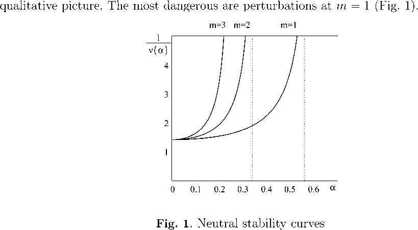
Using the obtained formulas, we construct graphs of curves of neutral stability y =

. For general flows, as well as for special cases considered above, there is a similar ^v(a)

The found asymptotics allows us to investigate the trajectories of the motion of passive impurity particles in the secondary self-oscillatory flow [8]. The trajectories of particles in the linear approximation satisfy the equation x = V (x) + u(x, t), u(x, t) = tpei^ +

The qualitative behavior of the trajectories is presented in Fig. 2.

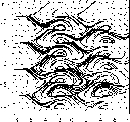
Fig. 2 . Trajectories of the motion of particles of a passive admixture

Conclusion

The first terms of the long-wavelength asymptotics with respect to the parameter α of linear spectral problem for a class of non-parallel flows close to the shear are found. A comparison with the case of the shear basic flow is made. It is shown that the expansion coefficients in terms of α eigenvalues and the critical value of viscosity have the form (17), where the square brackets are used to denote the coefficients of viscosity and eigenvalues in the case of basic shear flow, and the wave is used to denote additional term. If V1(z) = 0 then that additional term is equal to zero.

The first terms of the expansion in series in the parameter a of velocity v 0 (z) , v0(x, z) , v1(x, z) and pressure P 0 , P ¹ coincide with the coefficients for the case of shear basic flow. Average values ( v1 Y = ( vl Y = 0 , as in the case of shear basic flow, but ( v k ) = 0 for k ^ 3 .

The coefficients of the decomposition in a series of eigenfunctions have the following structure:

vk = [vk ] + vk + ^1({^k-1>) + (vk y vk = [vk ] + vk + v2((vk-1Y) + v2 ((vk>), and the coefficients of decomposition in a series of pressure have the following structure p k = [pk ] + pk + p 1({vk-1)) + (p k Y

Here k = 1, 2, 3,4 . The expressions in square brackets [v k ] , [P^k ] are the solutions of the same equations, as in the case of shear basic flow and coincide with corresponding coefficients if V j = 0 , o, = 0 .

If at least one of the conditions is met: 0(x) is odd or V1(z) is odd, then critical value of viscosity V 1 ( z ) is an even function of a as in the case of shear basic flow (up to order k = 4 inclusively):

v (a) = v * + V 2 a + V 4 a + O(a^ ),   a —— 0.

If 0(x) is odd, then odd components of the eigenvalue decomposition, starting with the third, are zero:

a(a) = ^i a + ^4 a + o^a^ + O(a ^), a —— 0.

If V 1 (z) is odd, then even components of the eigenvalue decomposition are zero:

^(a) = ^ia + ^з O' + ^5a⁵ + O(a^ ), a —— 0.

Thus, under both conditions eigenvalues up to terms of order α5 have the form a (a) = ±ima (V2) + O(a5), a — 0, as in a shear basic flow case.

For a basic flow close to a shear of general form the inequality v ₂ < [v ₂ ] is fulfilled, therefore, the loss of stability of such flows occurs at higher Reynolds numbers, than for shear flow.

Neutral stability curves qualitatively coincide with the corresponding curves for the Kolmogorov-flow (2). The trajectories of the passive admixture, found numerically, consistent with Obukhov’s hydrodynamics experiments [11].