On the Validity of Nonlinear and Nonsmooth Inequalities

Published Online January 2017 in MECS

There are some techniques that are frequently employed in proving inequalities. A method to prove the inequalities is to start from one side of the inequality and apply a sequence of known inequalities to reach the other side, or we may start from both sides and try to reach a common point. In fact, few problems concerning inequalities can be proved by a direct application of one of the most important and well-known inequalities. So, it is important to apply known inequalities suitably in order that the desired result can be obtained. Also, sometimes we deal with unapparent inequalities.

Several generalizations and proofs are given related to the inequalities, such as Jensen type inequalities [1-4], Hermite-Hadamard inequality [5-10], etc. But, it should always be remembered that there is no standard way of proof and there is no general rule in choosing techniques to be used. Specially, when we deal with inequalities including complicated nonlinear or nonsmooth terms, the proof is very hard. Also, when the number of variables appeared in inequalities is great, we usually do not obtain the validity of inequalities and prove them.

In the recent decades, optimization techniques and methods are developed in many fields and problems, but we do not see a technique based on optimization to prove the inequalities or to survey their validity. Hence, in this paper, an approach is presented to investigate the validity of the following general inequality using optimization:

F(X)≥0, X∈Ω             (1)

where F :Ω ⊂ ⁿ →      is a continuous function,

X — (XрX2?----,X^ ) and Q is a compact subset of n . Here, we do not know the inequality (1) is valid or invalid and there is not any approach to determine the validity of the general inequality (1).

• II.    M AIN I DEA

We consider the following problem corresponding to the inequality (1):

Minimize ^{F ( X )             (2)}

X ∈Ω

We note that since function F (.) is continuous and Q is compact, the optimization problem (2) has an optimal solution on Ω .

*

Theorem 2.1: Let X be the optimal solution of the optimization problem (2). The inequality (1) is valid when F ( X ^*) ≥0 .

*

Proof: Since X is the optimal solution of the optimization problem (2), for all X ∈ Ω , we have F ( X )≥ F ( X ^*) . So if F ( X ^*)≥0 then for all X ∈ Ω we have F ( X ) ≥ 0 , and this means inequality (1) is valid. Moreover, if F ( X ^*) < 0 then inequality (1) is invalid.

By considering the Theorem 2.1, from solving the optimization problem (2), we can recognize the inequality (1) is valid or invalid.

There are several well-known methods and algorithms for solving optimization problem (2), such as line search method, gradient method, Quasi-Newton Method, linearization method, steepest descent method, BFGS Method, etc. In the following, a good linearization method is given to solve the problem (2) in two cases: the function F (.) is smooth (continuously differentiable) or nonsmooth (nondifferentiable). By this method, we can obtain an approximate global optimal solution for smooth or nonsmooth optimization problem (2).

• A.    Linearization approach in order to solve the smooth optimization problem

In this subsection, assume that function F (.) has the continuous second order derivative. Divide the set Q to the similar grids Q_y , j = 1,2,..., m such that q = (J q. j = 1

and for all i ^ j , int(Q_z )Dint(Q) = Ф (where for every set A , the int( A ) shows the interior points of set A      ).      Select      the      arbitrary      points

Z. e int(Q_/.), j = 1,2,..., m , where m is a sufficiently big number. By Taylor expansion, for all X e Q^ , we have:

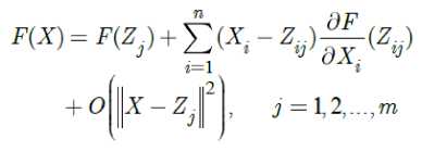
where

Z. — ( Z_VZ, .,...., Z .) j ^v 1 j ,   2 j ,     , nj^

and

X — ( X p X ₂,...., X_n ) . We can write for j — 1 , 2 ,..., m :

where —— rm - р^л +V - za—(zx

?=1i

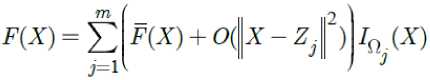
In (4), Р, (X) = 1 if, X eQ and in otherwise Qj

Ру ( X ) = 0 . By relation (4), we have

^Q j

But, by attention to the selected sets

Qj, j = 1,2,...,m and points Z^, j — 1,2,...,m , there exists sufficiency big number m0 eN such that for all m > m0

OГ|X-Z,II21< —,X eQ and -          11 J m hence, for sufficiently great number m , we can ignore the term

O -II X - 4

, X eQ j

for all

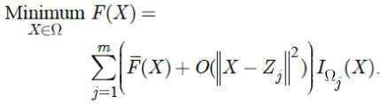
j — 1, 2,..., m . Hence, the minimization problem (2)

can be converted to the following minimization:

Minimize ^teQ

J=1        3

where m is a sufficiently big number and function F (.) is defined by (5). Thus, by solving nonlinear programming (NLP) problem (6), we can reach to an approximate optimal solution for (2). In below, is shown that by solving some linear programming (LP) problem, we can obtain the optimal solution of NLP problem (6).

Theorem 2.2: Let X^j ’* ( /' — 1,2,..., m ) be the optimal solution of the following linear programming (LP) problem:

n

Minimize F ( X ) = F ( Z j ) + £ ( X i. - Z j )—( Z j )

j                                              i = 1

where Z j = ( Z 1 j , Z ₂ j ,..., Z_nj ) eQ j is given and X — ( X p X ₂,...., X_n ) is the variable of the problem. Further, suppose that

F(Xp’*) — Minimum F(X^,*).

j — 1 , 2 ,..., m

Then X p ^p is a global optimal solution for the NLP problem (6).

Proof: Let X eQ be an optimal solution for the NLP problem (6), X ^ X p ,* and F ( X ) <  F ( X^p ,* ) . So there is k e {1,2,..., m } such that X e Q and

I Fk^ = Minimum F^X^

F(X) = Minimum F(X\But о, сП,soF(Xp") = Minimum F(X'").

j = 1,2,... m

Hence,

F ( X^k ’* ) — F ( X ) .              (8)

On           the           other           hand,

F(Xp’*) — Minimum F(Xj’*) and j — 1,2,..., m

F ( X p ,* ) <  F ( X^k ," )              (9)

By (8) and (9), we have F ( X^{p ,*}) ≥ F ( X^{k ,*}) which is a contradiction.

Remark 2.1 : By Theorem 2.2, we solve the LP problem (7), for j = 1, 2,.... m , to obtain the optimal solution of the NLP problem (6). We note that, for sufficiently number m , the optimal solution of the NLP problem (6) is an approximate optimal solution for the NLP problem (2). Moreover, by Theorem 2.1, the optimal solution of the optimization problem (2) shows that smooth inequality (1) is valid or invalid.

• B.    Linearization approach in order to solve the nonsmooth optimization problem

We suppose that function F (.) is continuous but nonsmooth (or nondifferentiable) on W . Hence, the problem (2) is a nonsmooth optimization. In this paper, the practical generalized derivatives (GDs) and generalized first order Taylor expansion (FOTE) of nonsmooth functions proposed by Noori Skandari et.al. (see [11,12]) is used to solve the nonsmooth optimization problem (2). A similar approach is given [13] to solve the nonsmooth optimization problems. Also, some other types of GDs are presented in [14,15].

As the following, the GDs and generalized FOTE are introduced at first, and then they are utilized to solve the nonsmooth optimization problems (1).

Assume C(Ω) is the spaces of continuous and continuous differentiable functions on the set Ω . Let ϕ(.), j = 0,1,2,... are the continuously differentiable basic functions for the space C(Ω) and suppose N(S) is the neighborhood of S with the radius δ . In addition, selecting the arbitrary points S ∈int(Ω) i = 1, 2,...,m where the sets ^ = (I = 1,2,..., m) are defined in subsection 2.1. Now, consider the following optimization problem:

Minimize ajkeR

W

FQCpF^- zSt^-^w^)

t=l 7=0

dX

where δ > 0 is a given sufficiently small number, X = ( X 1 ,.., X n ) and S = ( S_lY,...,S„ ) e int(Q) for all i = 1, 2,... , m . By assumption

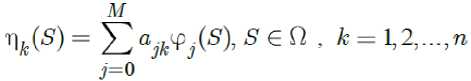
^c?) = Eajk^As^ Sc^-k=^^-^n- k = 1, 2,...,n , the problem (10) is equivalent to the following problem:

Minimize чк(-^с^

Now, let ( η ^*(.),..., η ^*(.)) be the optimal solution of the optimization problem (11). The GD of the function F (.) with respect to X is denoted by d_xF (.) and defined as d_x^F ( S_; ) = Пк(Si ) for k = 1, 2,..., n and i = 1, 2,..., m (see [6,7]). Here, by assumption

(where M is a sufficiently big number), the infinite dimensional nonsmooth optimization problem (11) can be approximated to the following finite dimensional smooth problem (see [12]):

Minimize f v^X^S^dX

Ч-Л,а-Зк I=1 N /g\

subject to-«(^spxFW-FtS,)

- X ^k - ^ik^jk^j^d k=l j=0

-^,sf)< -F(X) + F(S,)

+ S 52 ^^xk - s.X^M^ k=\ j=0

i = l,2,...,m, X E Q.

Further, in [11,12] is showed that this smooth problem can be approximated to a LP problem. Hence, the GD of nonsmooth      function       F (.)        is       as

∑*

a ^* _jkϕ_j (.), k =1,2,..., n where a_jk (for all k and j ) is the optimal solution of the linear optimization problem (12). In [12] is showed that the best linear approximation of the continuous nonsmooth function F (.) , in passing of point S_t e int(Q) , is as follows:

F(X) = F^ + E (X - 8_гк)Э_х^(8_г)

where dxF(Si) = f»y(Sj) for k = 1,2,... ,n j=0

and, ak for j = 0,1,..., M and k = 1, 2,..., n are the optimal solutions of the problem (12). Further, in [12] is      showed      that      the      total      error

Fff (,)(.) = ||f (.) - F (.)|| n5 (s)       of       the approximation F(.) F(.) on N(S), tends to zero when 5 ^ 0 . Also, the generalized FOTE of the continuous nonsmooth function F : Q C R” ^ R is given as follows:

F^FiSJ + t^-S^d MS,)

+ S,№)W. xe№6(S,), where E(X) is the pointwise error of the approximation F(X) « F(X) , X E N5 (S ) (the function F(.) is defined by (13)).

By generalized FOTE, the minimization problem (2) lead to the following minimization:

X = ( X p X 2,...., X_n ) . Further, suppose that

F(Xp,*)= Minimum F(Xi,*).

i = 1 , 2 ,..., m

Then X^p ’* is the global optimal solution of the NLP problem (15).

Proof: The proof is similar to the proof of Theorem 2.2.

Remark 2.2: By above theorem, we solve the LP problem (16), for i = 1, 2,.... m , to obtain the optimal solution of the NLP problem (15), and then obtain an approximate optimal solution for the nonsmooth optimization problem (2) to determine the validity of nonsmooth inequality (1).

• III.    S IMULATION RESULTS

In this section, the results and efficiency of presented approach be simulated in some examples.

Example 3.1 : We survey the validity of the following smooth inequality:

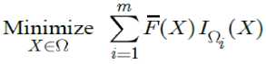
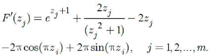
e^+l _p ^^zp2 + 1) ^ ж2 +2 sin^tz?) + 2 cos(tv^) , x E [0Л].

We define

F^x) = ez+1 + Ln(x2 +1)— ж2 — 2 sin(Tt^) — 2 соз^ж), x E [0,1]

and solve the NLP problem where m is a given sufficiently big number, linear function F(.) is defined by (13), and IQ.(.) is characteristic function of set Q .

Theorem 2.3: Consider the NLP problem (15). Let i ,*

X  (i = 1, 2,...,m) be the optimal solution of the following linear programming (LP) problem:

Minimize

F(X) = F(S_t) + E(^ - 8_гз)д_х F(S_l3),

Minimize F(x) subject to 0 < x < 1

For applying the linearization approach stated in

Section 1.2, we assume that m = 1000 and

Qj =

z

j

^, mm

2j -  1

2n

j = 1,2,

m and select points

, j = 1,2,...,m on

int(Q7) Now, the

corresponding LP problem (7) for j = 1, 2,..., m is as follows:

where        Si = (Si 1,..., S^ )        is        given,

X = ( X 1 , X ₂ ,...., X n ) is the variable of the problem, and d_x F (.) is the GD of F (.) with respect to

Minimize F^x) = F^3 ) + (ж - z3 )F\z3 )

subject to ----< x < —, m     m

where

By solving the LP problem (19), we obtain the optimal j solution XJ, , j — 1, 2,..., m. Moreover, we have

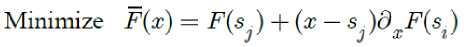
Minimum F(xj, )— F(xp, )— 0.4651542. j —1,2,..., m where xp, — 0.1360000 is an approximate global optimal solution for the smooth NLP problem (20). Thus, by attending to Remark 1.2, since F(x) ≥ 0.4651505 >0 the inequality (18) is valid. Here, the graph of functions F(.) and F'(.) are showed in Figure 1.

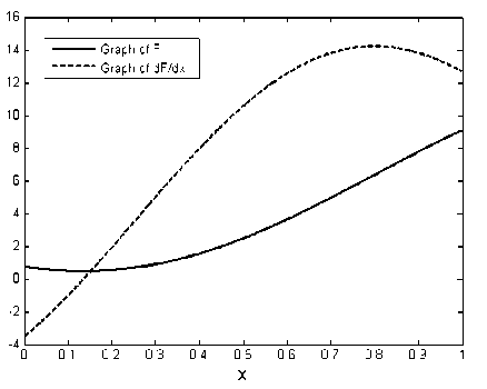
Fig.1. Graph of function F (.) and its GD in Example 3.1.

Example 3.2 : We show that the following nonsmooth inequality is invalid:

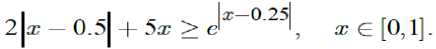
We define

F($) — 2|$ — 0.5| + 5ж — J I, $€[0,1], and assume that m — 1000 and ^ = [----, —] , mm

2i - 1

i — 1, 2,...,m . Also, we select points S- — -------, im i — 1, 2,..., m - 1 on int(Q). We first calculate the GD of nonsmooth function F(.) defined by (21). For this goal, we discrete the corresponding continuous optimization problem (12) the same as works [11,12]. After this discretization, we reach to a LP problem and by solving of which we obtain GD of F (.) as ∂F(s ),i =1,2,...,m , where it is illustrated in Figure 2. Now, we solve the nonsmooth NLP problem

• ■ ■ ■ Z X I             I                  It— 0.25|

Minimize F^x) = 2 ж — 0.5 + 5ж — e 1

s ubject to 0≤ x ≤1               (22)

Here, the corresponding LP problem (16) for i — 1, 2,..., m is as follows:

subject to       ≤ x ≤                  (23)

mm

By solving the LP problem (23), we obtain the optimal j, solution XJ  , j — 1, 2,...,m. Moreover, we have

Minimum F(xj, ) — F(xp, ) j — 1,2,..., m

— - 0.2840252 < 0

where x^{p ,*} =0.5×10 ^{- 16} is an approximate global optimal solution for the nonsmooth NLP problem (22). Thus, by attending to the Remark 2.2, the inequality (20) is invalid.

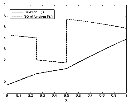
Fig.2. Graph of function F (.) and its GD in Example 3.2.

Example 3.3 : We survey the validity of the following nonsmooth inequality:

Зх^ + 2|ж| — ж2| + 0.5 >

1.5ж₂ + ж^ |sin(it(x₂ — 0.75)|, ЖрЖ₂ £ [0,1]².

Assume that

F(x. , ж-) = Зж, ж- + 2 ж. — ж₇

• — 1.5ж₂ — ж₁ sin(it(x₂ — 0.75)| + 0.5,

ЖрЖ2 € [0,1]2, and solve the following nonsmooth NLP problem:

Minimize F(x^, х_э)

subject to 0 <  ж^ < 1, 0 <  х^ < 1.

For this purpose, we assume that m — 200 and

Ц, = [ — , — ]x[j-1,j], for i — 1,2,...,m and mm mm j — 1,2,...,m     .     Also,      select     points

2 i -1   i 2 j -1 j

(si,sj)=(       ,   ]×[       ,   ) ∈int(Ωij) . we mm mm first calculate the GD of nonsmooth function F(.) defined by (25) where it is illustrated in Figure 3. By discretization the corresponding continuous optimization problem (16), we reach to the some LP problems and obtain the GD of F(.) with respect to X^ and X^ as dx 1 F(si,sj) and dx2F(si,sj), for i — 1,2,...,m and j — 1,2,...,m , where they are illustrated in Figures 4 and 5, respectively. Now, the corresponding LP problem (16), for solving the nonsmooth NLP problem (26), is as follows (for i — 1,2,...,m   and j — 1,2,...,m ):

Minimize F(xpx2)— F(st,s^)

+ (ж. — s)S F(s.,s + (x₉-s )5 F(s-,S.) з> х-j ^x г’ j'

, . i — 1 ,      , i i — II _ subject to ----< ж. < —, ----< Xy < —,

'   m    mmm

By solving the LP problem (27), we obtain the optimal solution ( X^ , xj ) for i — 1,2,..., m and j — 1, 2,..., m . Moreover, we have

Minimum F ( x^ * , x₂^j * ) — F ( x ^* , x, q * ) i , j — 1,2,..., m

— 0.0004391>0

where ( x? * , x^ * ) — (0.3524999,3524999) is an approximate global optimal solution for the nonsmooth NLP problem (26). Thus, by attending to the Remark 2.2, the inequality (24) is valid.

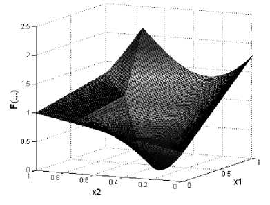
Fig.3. The graph of function F(.,.) for Example 3.3.

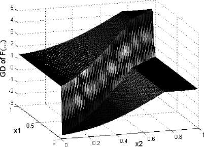
Fig.4. The graph of ∂ F (.,.) for Example 3.3.

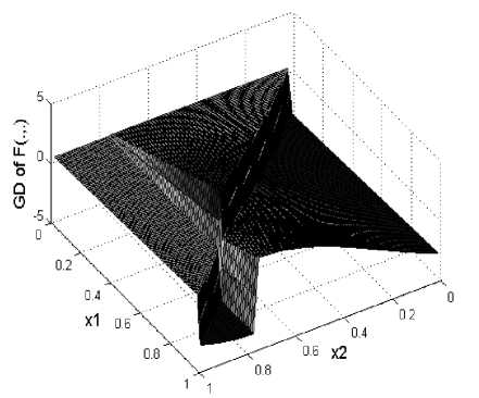
Fig.5. The graph of ∂ F (.,.) for Example 3.3