Определение абсолютного полного электронного содержания по одночастотным спутниковым радионавигационным данным GPS / ГЛОНАСС

Автор: Ясюкевич Ю.В., Мыльникова А.А., Иванов В.Б.
Журнал: Солнечно-земная физика @solnechno-zemnaya-fizika
Статья в выпуске: 1 т.3, 2017 года.
Бесплатный доступ
В работе представлен новый подход, позволяющий произвести оценку абсолютного вертикального и наклонного полного электронного содержания (ПЭС) ионосферы. Оценка основана на использовании одночастотных совместных измерений фазового и группового запаздывания сигнала GPS/ГЛОНАСС по данным отдельных измерительных станций. Качественно и количественно вертикальное ПЭС, рассчитанное по одночастотным измерениям, согласуется с аналогичными оценками, основанными на двухчастотных измерениях. Типичное значение разности вертикального ПЭС, полученного одночастотным и двухчастотным методом, для выбранных нами станций в основном не превышает величины ~1.5 TECU с СКО до ~3 TECU.
Ионосфера, глонасс, полное электронное содержание, одночастотные данные
Короткий адрес: https://sciup.org/142103636
IDR: 142103636 | УДК: 550.388.2 | DOI: 10.12737/23509
Текст научной статьи Определение абсолютного полного электронного содержания по одночастотным спутниковым радионавигационным данным GPS / ГЛОНАСС
The first studies to assess the daily dynamics of the total electron content (TEC) in the ionosphere based on data from global navigation satellite systems (GNSS) were published in the late 1980s. [Lanyi, Roth, 1988]. The evolution of this line of research, on the one hand, led to the development of Global Ionospheric Maps (GIM) [Schaer et al., 1998a; Manucci et al., 1998; Hernandez-Pajares, 2009], which, in turn, significantly advanced ionospheric research [Afraimovich et al., 2008; Liu et al., 2009; Hocke, 2008; Lean et al., 2011; Gulyaeva, Veselovsky, 2012; Cherniak et al., 2014], and, consequently, stimulated the development of new ionospheric models [Ivanov et al., 2011]. On the other hand, a large number of studies to determine the vertical TEC at an individual station have been carried out [Durmaz, Karslioglu, 2015; Themens et al., 2015; Yasyukevich et al., 2015], which provided extensive data to elaborate the ionospheric models [Gulyaeva, 2016; Themens, Jayachandran, 2016].
In most of the studies, TEC was estimated using data from dual-frequency (L1, L2) radionavigation receivers. The algorithm for single-frequency data is well known [Afraimovich, Perevalova, 2006; Mayer et al., 2008], but it has not gained widespread currency because of high noises of group measurements [Kunitsyn et al., 2007]. Although noises of group measurements are high enough, it can be expected that TEC estimates are quite adequate due to averaging. Accordingly, it is interesting to explore the possibility of determining TEC from single-frequency GNSS data. In 2012, Schuler, Oladipo [Schuler, Oladipo, 2012, 2014] implemented a scheme for determining vertical TEC from single-frequency measurements. Unfortunately, these articles do not describe in detail the algorithm for determining TEC, thus making it difficult to obtain similar results. In 2014, we proposed an algorithm Tay-AbsTEC for restoring the absolute vertical TEC [Mylnikova et al., 2014; Yasyukevich et al., 2015] as well as its gradients (linear and quadratic) and time derivatives (first and second), using dual-frequency measurements from an individual GPS/GLONASS station. With some minor modifications, this algorithm can be also applied to singlefrequency data. At the same time, along with the restoration of the absolute vertical TEC, it is possible to eliminate ambiguity from TEC measurements. As a result, absolute measurements can be made of slant TEC along satellite– receiver lines of sight. This can be used to solve applied problems of correcting the ionospheric effect on radio systems [Afraimovich, Yasukevich, 2008; Forte, Aquino, 2011; Ovodenko et al., 2015].
In this paper, we present a technique for determining absolute TEC, its gradients and time derivatives, as well as for eliminating ambiguities of measurements for some series of slant TEC along a satellite–receiver line of sight from single-frequency measurements.
TECHNIQUE FOR DETERMININGABSOLUTE IONOSPHERIC PARAMETERS FROM SINGLE-FREQUENCY DATA
To determine the absolute TEC, its gradients and time derivatives, as well as to eliminate ambiguity of measurements for series of slant TEC along a satellite–receiver line of sight using data from an individual GPS/GLONASS station, we have adopted the following algorithm similar to that applied to dual-frequency observations [Yasyukevich et al., 2015].
-
1. Calculation of slant TEC ( I P φ ) from simultaneous group and phase measurements:
-
2. Separation of data series into continuous time intervals. This stage is quite important since the phase ambiguity during data discontinuity usually changes. Maximum length of the series is limited by the time of satellite observation and can be as long as ~8 hours. The minimum length of a continuous interval is chosen arbitrarily. In the implemented algorithm, a series with a 30-s time resolution should contain at least 10 measurements.
-
3. Detection and elimination of the impact of outliers and cycle slips in TEC data [Blewitt, 1990].
-
4. Evaluation of the absolute vertical TEC, its gradients, and time derivatives with a simple measurement model. Ambiguity in measurements K is estimated at a time. Parameters of the model are determined by minimizing the root mean square (RMS) of experimental and modeled data (see below).
-
5. Elimination of ambiguity from slant TEC data obtained in Section 3.
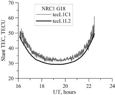
Figure 1 shows initial (without eliminating ambiguity and outliers) series of slant TEC obtained from singlefrequency (gray curve) and dual-frequency (black curve) measurements at the NRC1 station (45.5° N, 104.4° W). It can be seen that the TEC series derived from single-frequency data is characterized by a high noise level. Nevertheless, the form of the series is very similar. This is to be expected provided that receiver measurements are correct and there is no strong receiver clock bias. Noises of measurements if they are uncorrelated and have no systematic component should not play a big role because with RMS minimized, the solution should become optimal.
Ipm =-----Г( P - L M + K + aLP 1 , (1)
Pф 2 40.308LV 1 1 17 J where f1 is the main operating GNSS frequency (GPS, GLONASS, or others); P1 is the additional radio propagation path that is associated with the ionospheric group delay and calculated from P1- or C1-code, m; L1λ1 is the additional radio propagation path associated with the phase delay in the ionosphere, m; L1 is the number of phase rotations at the main GNSS frequency; λ1 is the wavelength, m; K is the constant value determined by the ambiguity of phase measurements and the time of signal propagation in satellite and receiver equipment; aLP are total noises of phase and group measurements at the main frequency. The elevation cutoff is 10°. Simultaneously with the computation of the TEC series, we calculate elevation angles and azimuths of satellites. The calculation is performed for both GPS and GLONASS data, no distinctions made then between GPS and GLONASS data.
Figure 1 . Slant TEC series derived from single-frequency (gray curve) and dual-frequency (black curve) measurements made at the NRC1 station (45.5° N, 104.4° W) using G18 GPS satellite data
In general terms, the measurement model of slant TEC I M has the following form:
I M = S j V ( Ф , l , t ) + I k ,j
where ϕ is the geographic latitude of the ionospheric point – the point of intersection of the satellite–receiver line of sight with the ionosphere at a height of 450 km, l is the geographic longitude of the ionospheric point. The index i is put into correspondence with the discrete measurement time and j into correspondence with the number of continuous interval (separately for each satellite and each continuous interval), I V is the absolute vertical TEC, I K is the constant for a continuous interval associated with ambiguity in phase measurements and signal delay in receiver and satellite paths, S i is the oblique factor in the approximation of a thin, single-layer ionosphere.
In this article, we focus on the oblique factor used in [Yasyukevich et al., 2015]
Sj =
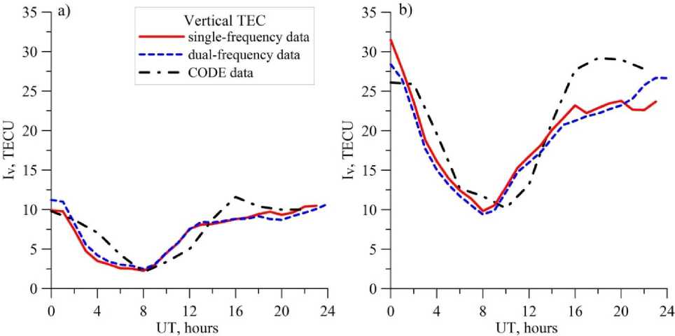
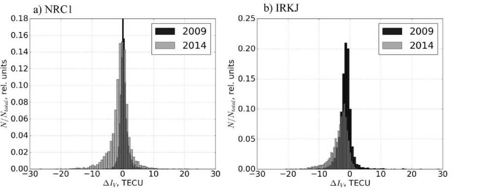
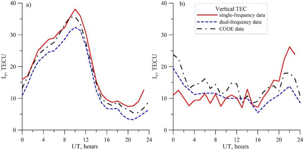
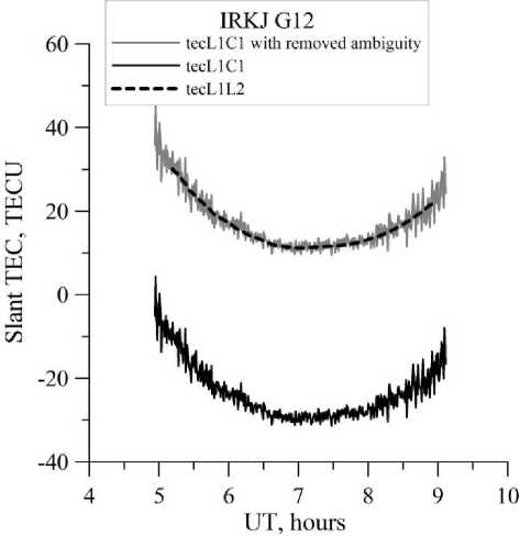
I I R • r cos I I RE +hmax -1 where RE is the Earth radius, hmax is the height of the thin spherical layer (450 km), a=0.97, 0j is the satellite eleva- tion angle. Using the Taylor expansion at the point (ϕ0, l0, t0), we can write to to to IV (ф, i, t )=Z2Z m=0 n=0 k=0 (Аф)m (Al)n (At)k дm+n+kIV m! n! k! дфm дln дtk, where Δ ϕ is the difference in latitude between coordinates of the ionospheric point and station ϕ 0; Δl is the difference in longitude between coordinates of the ionospheric point and the station l0; Δt is the difference between measurement time and the time t0 involved in the calculation. Restricting ourselves to the first three terms [Yasyukevich et al., 2015], we get Im = Sj[Iv (Фо, lo, tо) + GфАфj + +Gq_ф(Аф‘)2+ GiAlj+ Gq_i (Alj )2+ (5) +GtAt'+ Gq_t (Atj)2] + Ik,j. Here, Gϕ=∂IV/∂ϕ, Gl=∂IV/∂l, Gq_ϕ=∂2IV/∂ϕ2, Gq_l=∂2IV/∂l2 are linear and quadratic spatial gradients of TEC; Gt=∂IV/∂t and Gq_t=∂2IV/∂t2 are the first and second time derivatives. Mixed space and time derivatives can be ignored if assumed that characteristic TEC gradients during the period involved in the calculation change more slowly than the vertical TEC itself. We simultaneously calculate the parameters for a full day for different moments of time tk, solving a compatible system of equations. To obtain parameters for each moment of time tk (t1 and t2 in Figure 2), we consider data for the interval of ±1 h relative to tk (see Figure 2). Arrows in Figure 2 indicate boundaries of the intervals related to t1 and t2. The interval that includes data from 6 to 8 UT pertains to t1; from 7 to 9 UT, to t2. As testing shows, the time resolution for the estimated parameters may be from several hours to 10 minutes. In this paper, we present parameters with a time resolution of 1 hr. This choice stems from the fact that the maximum resolution of GIM maps is 1 hr. Figure 2. Contribution of measurements of individual satellites to estimates of vertical TEC at different moments of time The system of equations derives from minimizing functional (6) for each selected tk, for which the parameters are estimated by least squares: и*=ts“jiMi-1„ ■ j=1 i=1 to *, J= to * (tj) = @( t* -t' + At) x i Г ( at‘, * Y x0(t'+At - tk)— 1 + —J— Si I A t J where Iexp are experimental single-frequency measurements of slant TEC made after stage 3 of the algorithm; Θ is the Heaviside function; tj is the i-th instant of j-th satellite measurement; AtJ * is the time difference between the current measurement and the time tk involved in the calculation; Δt=1 h is the maximum time difference at which the data are still used to estimate the current ionospheric parameters. The presence of the multiplier 1/S in (7) leads to the fact that the greatest contribution comes from measurements at large satellite elevation angles. Differentiating (6) from each of the parameters of model (5) IkV, Gkϕ, Gkl, Gkq_ϕ, Gkq_l, Gkt, Gkq_t, IK for each instant, we obtain a system of 7J+M equations (J is the number of instants in the interval of interest involved in the calculation, M is the number of continuous intervals for all observed satellites). EXPERIMENTAL RESULTS For the analysis, we have used data from the dual-frequency receiver network IGS [Dow et al., 2009] in the Asian and American sectors of the Northern Hemisphere (the IRKJ (52.2° N, 104.3° E), NRC1 (45.5° N, 104.4° W), and YELL (62.5° N, 115.5° W) stations). This enabled us to obtain TEC estimates not only with the algorithm for single-frequency measurements but also with the similar technique TayAbsTEC for simultaneous dual-frequency phase and group measurements [Yasyukevich et al., 2015]. Figure 3 depicts the results of the above described algorithm in comparison with the results obtained with TayAbsTEC. This figure also presents vertical TEC data from global ionospheric maps GIM of the CODE laboratory [Schaer et al., 1998a], available on the website [ftp://cddis.gsfc.nasa.gov/gps/products/ionex/] in IONEX format [Schaer et al., 1998b]. The time resolution is 1 hr for data from a single station and 2 hr for GIM data. Referring to Figure 3, the dynamics of the vertical TEC obtained by different methods is qualitatively and quantitatively the same. At the same time, as, say, for May 20, 2014 (Figure 3, b), we can have a difference over 2 TECU. In some cases, there are more significant errors between single-frequency and dual-frequency data. The difference with CODE data is commonly greater. To evaluate the possible error, we computed the distribution of differences between values acquired from single-frequency and dual-frequency measurements. To do this, for each of the days of 2009 (minimum solar activity) and 2014 (maximum solar activity) we calculated series of the absolute vertical TEC from singlefrequency and dual-frequency measurements, using GPS/GLONASS IRKJ and NRC1 data. Then, we built a histogram of distribution of the difference between these parameters determined by the two methods. The time resolution in the calculation was 1 hr. The results are shown in Figure 4. The histograms are normalized to the total number of measurements Ntotal. Figure 3. Daily dynamics of TEC over the NRC1 station (45.5° N, 104.4° W) on May 20, 2009 (a) and May 20, 2014 (b) Figure 4. Histogram of distribution of the difference between vertical TEC obtained from single-frequency and dual-frequency measurements at the stations NRC1 (a) and IRKJ (b) in 2009 and 2014 For the NRC1 station, we can see a systematic component of ~0.5 TECU and a scatter with RMS of ~1.5 TECU for low solar activity, and ~ –0.5 TECU and ~ 3.5 TECU for high solar activity. For the IRKJ station, these values are higher: the systematic component is ~ –1.5 TECU and RMS is ~ 2.5–3 TECU. Notice that the values of the difference correspond as a whole to noises of initial measurements. Moreover, these errors (deviations) correspond in the order of magnitude to the systematic and random deviations of GIM maps of different laboratories. Accordingly, these deviations may be considered quite acceptable. A reason for the difference is likely to be the non-Gaussian shape and/or zero offset of group measurement error distribution. This issue requires an in-depth study. Another sufficiently important question concerns the efficiency of the algorithm under disturbed conditions, as well as its performance in a high-latitude region during irregular intense disturbances. We calculated the vertical TEC dynamics for the strong magnetic storm of March 17, 2015 [Astafyeva et al., 2015]. Figure 5 illustrates the daily dynamics of the absolute vertical TEC over the mid-latitude station IRKJ (52.2° N, 104.3° E) (a) and high-latitude station YELL (62.5° N, 115.5° W) (b). We can see that for middle latitudes the general dynamics is restored quite well. For high latitudes, the performance of the algorithm is significantly low, although it can still give acceptable results. In the test analysis carried out in a high-latitude region for a number of stations, we failed to obtain adequate TEC estimates. The possibility for estimating TEC at high latitudes depends on the data quality, which is generally worse at high latitudes than at middle ones. Cycle slips at high measurement noise levels strongly affect the quality of initial data in stage 4. This can make it impossible to derive an adequate solution. The development of the proposed technique can go toward improving the preprocessing of initial TEC series and toward reducing the influence of cycle slips and measurement noises. Figure 5. Daily dynamics of the absolute vertical TEC over the mid-latitude station IRKJ (a) and the high-latitude station YELL (b) during the strong magnetic storm of March 17, 2015 Figure 6 sheds light on how to obtain absolute values of slant TEC. Here, we present initial single-frequency TEC measurements (black solid line), single-frequency TEC measurements after disambiguation (gray curve), as well as dual-frequency measurements of phase TEC with phase ambiguity eliminated (dashed curve). The figure shows data for May 11, 2009. It can be seen that for the chosen satellite the corrected measurements are positive definite compared to initial measurements. Finite measurements here are “pure” measurements with no filtering effects. The figure demonstrates agreement between single-frequency and dual-frequency measurements of slant TEC after disambiguation. After being smoothed, single-frequency data can be used to correct ionospheric models or to solve a number of practical problems. Figure 6. Slant TEC along the G12 GPS satellite–IRKJ station line of sight, May 11, 2009 CONCLUSION We believe that the technique for obtaining absolute TEC values from single-frequency measurements can promote the development of ionospheric monitoring, especially in the Russian Federation, where the number of dualfrequency receivers is not as great as, for example, in Japan or the United States. As our analysis shows, singlefrequency measurements of vertical TEC rank only slightly below dual-frequency measurements in quality. A restriction on the use of this technique for single-frequency GPS/GLONASS equipment is that the quality of phase and group measurements with general-purpose receivers can be lower than those with special-purpose IGS equipment. Accordingly, in the future we plan to estimate the effect of noise level on data quality as well as to compare noise characteristics of general- and special-purpose receivers. We are grateful to Padokhin A.M. for useful discussion and valuable comments. We appreciate the IGS network [Dow et al., 2009] for providing the GPS/GLONASS data used in this work. This work was supported by RFBR grant No. 16-35-00051, as well as RF President Grant of Public Support for RF Leading Scientific Schools (NSh-6894.2016.5).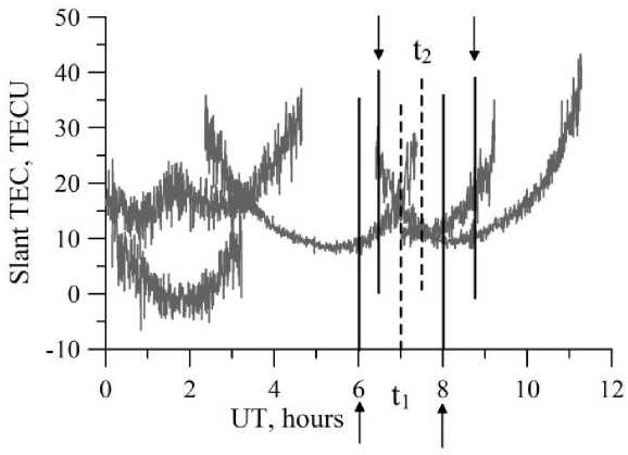
Список литературы Определение абсолютного полного электронного содержания по одночастотным спутниковым радионавигационным данным GPS / ГЛОНАСС
- Афраймович Э.Л., Перевалова Н.П. GPS-мониторинг верхней атмосферы Земли. Иркутск: ГУ НЦ ВСНЦ СО РАМН, 2006. 480 с.
- Гуляева Т.Л. Модификация индексов солнечной активности в международных справочных моделях ионосферы IRI и IRI-Plas в связи с пересмотром ряда чисел солнечных пятен//Солнечно-земная физика. 2016. Т. 2, № 3. C. 59-68 DOI: 10.12737/20872
- Куницын В.Е., Терещенко Е.Д., Андреева Е.С. Радиотомография ионосферы. М.: Физматлит, 2007. 255 с.
- Мыльникова А.А., Ясюкевич Ю.В., Демьянов В.В. Определение абсолютного вертикального полного электронного содержания в ионосфере по данным ГЛОНАСС/GPS//Солнечно-земная физика. 2014. Вып. 24. С. 70-77.
- Ясюкевич Ю.В., Мыльникова А.А., Куницын В.Е., Падохин А.М. Влияние дифференциальных кодовых задержек GPS/ГЛОНАСС на точность определения абсолютного полного электронного содержания ионосферы//Геомагнетизм и аэрономия. 2015. Т. 55, № 6. С. 790-796 DOI: 10.7868/S0016794015060176
- Afraimovich E.L., Yasukevich Yu.V. Using GPS-GLONASS-GALILEO data and IRI modeling for ionospheric calibration of radio telescopes and radio interferometers//J. Atmos. Solar-Terr. Phys. 2008. V. 70, N 15. P. 1949-1962.
- Afraimovich E.L., Astafyeva E.I., Oinats A.V., et al. Global electron content: A new conception to track solar activity//Ann. Geophys. 2008. V. 26, N 2. P. 335-344. DOI: 10.5194/angeo-26-335-2008.
- Astafyeva E., Zakharenkova I., Foerster M. Ionospheric response to the 2015 St. Patrick's Day storm: A global multi-instrumental overview//J. Geophys. Res. Space Phys. 2015. V. 120, N 10. Р. 9023-9037 DOI: 10.1002/2015JA021629
- Blewitt G. An automatic editing algorithm for GPS data//Geophys. Res. Lett. 1990. V. 17. P. 483-492.
- Cherniak I., Zakharenkova I., Krankowski A. Approaches for modeling ionosphere irregularities based on the TEC rate index//Earth, Planets and Space. 2014. V. 66. P. 165 DOI: 10.1186/s40623-014-0165-z
- Dow J.M., Neilan R.E., Rizos C. The International GNSS Service in a changing landscape of Global Navigation Satellite Systems//J. Geodesy. 2009. V. 83. P. 191-198 DOI: 10.1007/s0019000803003
- Durmaz M., Karslioglu M.O. Regional vertical total electron content (VTEC) modeling together with satellite and receiver differential code biases (DCBs) using semi-parametric multivariate adaptive regression B-splines (SP-BMARS)//J. Geodesy. 2015. V. 89, iss. 4. P. 347-360. DOI 10.1007/s00190-014-0779-8.
- Forte B., Aquino M. On the estimate and assessment of the ionospheric effects affecting low frequency radio astronomy measurements//Proc. 30th URSI General Assembly and Scientific Symp. 2011. P. 1-4.
- Gulyaeva T.L., Veselovsky I.S. Two-phase storm profile of global electron content in the ionosphere and plasmasphere of the Earth//J. Geophys. Res. 2012. V. 117. A09324 DOI: 10.1029/2012JA018017
- Hernández-Pajares M., Juan J.M., Sanz J., et al. The IGS VTEC maps: A reliable source of ionospheric information since 1998//J. Geodesy. 2009. V. 83: Special IGS Issue. P. 263-275 DOI: 10.1007/s00190-008-0266-1
- Hocke K. Oscillations of global mean TEC//J. Geophys. Res. 2008. V. 113. A04302 DOI: 10.1029/2007JA012798
- Ivanov V.B., Gefan G.D., Gorbachev O.A. Global empirical modelling of the total electron content of the ionosphere for satellite radio navigation systems//J. Atmos. Solar-Terr. Phys. 2011. V. 73. P. 1703-1707.
- Lanyi G.E., Roth T. A comparison of mapped and measured total ionospheric electron content using Global Positioning System and Beacon satellite observations//Radio Sci. 1988. V. 23, N 4. P. 483-492 DOI: 10.1029/rs023i004p00483
- Lean J.L., Emmert J.T., Picone J.M., Meier R.R. Global and regional trends in ionospheric total electron content//J. Geophys. Res. 2011. V. 116. A00H04 DOI: 10.1029/2010JA016378
- Liu L., Wan W., Ning B., Zhang M.-L. Climatology of the mean total electron content derived from GPS global ionospheric maps//J. Geophys. Res. 2009. V. 114. A06308 DOI: 10.1029/2009JA014244
- Mannucci A.J., Wilson B.D., Yuan D.N., et al. A global mapping technique for GPS-derived ionospheric TEC measurements//Radio Sci. 1998. V. 33, iss. 3. P. 565-582 DOI: 10.1029/97RS02707
- Mayer C., Jakowski N., Beckheinrich J., Engler E. Mitigation of the ionospheric range error in single-frequency GNSS applications//Proc. 21st Intern. Technical Meeting of the Satellite Division of the Institute of Navigation (ION GNSS 2008), Savannah, GA. 2008. P. 2370-2376.
- Ovodenko V.B., Trekin V.V., Korenkova N.A., Klimenko M.V. Investigating range error compensation in UHF radar through IRI-2007 real-time updating: Preliminary results//Adv. Space Res. 2015 DOI: 10.1016/j.asr.2015.05.017
- Schaer S., Beutler G., Rothacher M. Mapping and predicting the ionosphere//Proc. IGS AC Workshop. Darmstadt, Germany, 1998a. P. 307-320.
- Schaer S., Gurtner W., Feltens J. IONEX: The ionosphere map exchange format Version 1//Proc. IGS AC Workshop, Darmstadt, Germany. 1998b. P. 233-247.
- Schuler T., Oladipo O.A. Single-Frequency GNSS Ionospheric Delay Estimation -VTEC Monitoring with GPS, GALILEO and COMPASS: 1st edition. Lulu Press, 2012.
- Schuler T., Oladipo O.A. Single-Frequency single-site VTEC retrieval using the NeQuick2 ray tracer for obliquity factor determination//GPS Solution. 2014. V. 18. P. 115-122 DOI: 10.1007/s10291-013-0315-y
- Themens D.R., Jayachandran P.T. Solar activity variability in the IRI at high latitudes: Comparisons with GPS total electron content//J. Geophys. Res. Space Phys. 2016. V. 121. P. 3793-3807 DOI: 10.1002/2016JA022664
- Themens D.R., Jayachandran P.T., Langley R.B. The nature of GPS differential receiver bias variability: An examination in the polar cap region//J. Geophys. Res. Space Phys. 2015. V. 120. P. 8155-8175 DOI: 10.1002/2015JA021639
- URL: ftp://cddis.gsfc. nasa.gov/gps/products/ionex/(дата обращения 12 декабря 2016 г.).
