Optimal Control of Switched Systems based on Bezier Control Points

Published Online June 2012 in MECS

A switched system is composed of some subsystems and a switching law. The switching law defines the order of the subsystems which have to be activated at specified switching instants during the planning horizon. Many real world applications face switched systems, such as the control of mechanical systems, automotive industry, aircraft and air traffic control and switching power convertors (details can be found in [1-7]).

The objective of problems related to optimal control of switched systems is to find a switching law and a control function in a way that some performance criteria are minimized with respect to imposed constraints on state and control variables. These groups of optimal control problems are of theoretical and practical importance, so they have been taken into special consideration ([8-12]).

For switched system with linear component systems, the defect of optimal control switching has absorbed several researcher's attention recently. For instance, Egerstedt, et al. [13] presented such an accurate method and algorithm that is able to compute the minimum number of switching for changing from one state to another and Xu, and Antsakalis [14], addressed the problem of determining the switch instants.

These results, like most of the results in the literature, make open-loop and are based on pre-selecting a finite number of switching and optimization of the switching instance against a cost functional. For these open-loop solutions, the result of optimization can be enhanced if the number of switching is allowed to increase but since these methods use a search algorithm, the cast of computation increases very suddenly. Xu, and Zhai [15] continued their recent study on practical stabilizability of discrete-time (DT) switched systems, and they proved a sufficient condition for Е -practical asymptotic stabilizability. On the basis of their approach, they also presented several new sufficient conditions for global Е -practical asymptotic stabilizability of such a class of systems.

Niua, and Zhaoa [16] surveyed the problem of stabilization and ^2 -gain analysis for a class of cascade switched nonlinear systems by using the average dwelltime method. First, when all subsystems were stabilizable, they designed a state feedback controller and an average dwell-time scheme, which guaranteed that the corresponding closed-loop system was globally asymptotically stable and had a weighted ^2 -gain. Then, they extended the result to the case where not all subsystems were stabilizable, under the condition that the activation time ratio between stabilizable subsystems and unstabilizable ones was not less than a specified constant, also they derived sufficient conditions for the stabilization and weighted ^2 -gain property.

In this work, a class of optimal switching problems have been considered such that the switching instants and the control function have to be found optimally under the condition of defined order of the subsystems. The purpose of this paper is to propose an efficient computational algorithm based on Bezier curves introduced in [3] for solving these type of optimal switching problems.

This paper is organized as follows: In Sections 2 and 3, the basic problem will be introduced. Two examples will be presented in Section 4 and solved by the proposed method. And at last, Section 5 will discuss about conclusion.

• II.    Switched Systems

A switched systems composing of following subsystems considered as follows:

• *(0 — F( t,x(t),u(t)),i e I — {1,2..... NY     (1)

• 5.    t. x(t) — F(x(t),u(t)), t e [to,A),(a)

where x(t) e R^p , u(t) e R^m and for each i e I,Ff.R ^p+m+1 ^ R ^p is continuously differentiable with respect to its arguments. To control a switched system, a continuous input as well as a switching sequence have to been selected. A switching sequence with t e [t_o, t y ] adjusts the order of active subsystems and is defined as:

о — {(To , i o ), ( АЛ).....( T_k, i_K}l          (2)

where 0 < К < “, to — To < A < — < TK < ty, and i k e 7 for k — 0,1, ...,K Here, (Tk, i k) indicates that at instant , the system switches from subsystem     to subsystem ik; therefore subsystem ik is active during time interval [Tk, Tk+^ ([Tk, Tk+1] if k — К). In order a switched system to be well-behaved, only nonZeno sequences are considered which switch at most a finite number of times in [t0, ty], though different sequences may be of different numbers of switchings. If is regarded as a discrete input, then the overall control input on the system is the pair (tr, it). It is mentioned that the discriminately factor for a switched system from a general hybrid system is its continuous state which doesn’t represent jumps at switching instants. Hence, the computation of continuous inputs becomes favorable via the application of conventional optimal control methods.

This paper goals at minimizing cost functional over two subsystems solution as the following form ft J mini—p).x( ty)/+ I  L(x(t),u(t))d t,

• x:(t) — G(x(t),u(O), te[Ti,ty],

x(t) — Ott, t < to, where         x(t) — ^(t) _xp(t))T e Rp, u(t) —

(it ₁(t)-U m (O)^T e R^m      ,       and       ф (t) —

(ф ₁(7)^ф_р(7))^т are known vectors functions, and t_o and t y are known values in R . We assume F(t) —

(А(Э -/р(.))Т andG(0 — (51(.) ^gp(.))T are vector functions, which their elements   assumed to be polynomials defined on [  ,  ) and [  ,  ], respectively.

We need to impose continuity on ( ) and its first derivative which these constraints is appeared in Section 3.

Without lose of generality just for simplicity, the case of two subsystems are considered in which the subsystems ( ) and ( ) in (3) are active in e [  ,   ) and e [  ,  ] , respectively ( is switching instant which has to be determined). Applying developed methods on problems with several subsystems with more than one switching is straightforward [14].

Problem (3) can be converted into a new problem. A state variable is introduced corresponding to switching instant T1. Let у satisfy

• 5 — 0,

• У (0) — A.

Now, a new variable f is introduced. Define a piecewise linear relationship between t and f as follows:

_ ( t₀ + ^(y - o))^, ⁰< ^f< 1

• t — {У+(ty - y)(f - 1), 1 < f < 2.

Obviously, f — 0 corresponds to t — to , f — 1 to t — У, and f — 2 to t — ty. By substituting у and ^ in (. ) and (. ) in equations ( ) and ( ) of (3), now these equations are converted  into the following equivalent forms:

^Xf2—(y-to)F 1(x(f)/u(O),

• 5 — 0,

where e [0,1) and

^— ( 0/-у)6 1(x(0,u(0),(9)

% — 0, where e [1,2], and

X(O — (oto + (y-to)O,f <0.

Now the target is to find and ( ), e [0,2]such that the cost functional

Remark 1: The equivalent problem (7)-(12) provides us with no more varying switching instant and consequently it is conventional. Since у actually is an unknown constant while f £ [0,2], thus у isregarded as unknown parameter for optimal control problem with cost (12) and subsystems (7)-(11), that is, Problem (7)(11) with cost functional (12) can be regarded as an optimal control problem parameterized by switching instant у. It is worth noting that by considering у as a parameter, thedimension of new problem is the same as that of first problem. In fact, this situation is valid when considering more than one switching.

• III.    Statement of Problem

Consider the optimal control of time varying system (7)-(11) with cost functional (12). Divide the interval [0,2] into a set of grid points such that ft = 0 + ih, i = 0,1, ..,k, where h = j, and k is a positive integer. Let St = [ f ;_ i, f/] for j = 1,2,—,k. Then, for f eSу the above optimal control problem can be decomposed to the following suboptimal control problems:

min / j   Cj + ft rs t ⁺ 4 eco n d

• s .t. Iftrst= I    Z[o,i) ⁽y-t oH OtpU^df,

e [0,1),

^second = I    Z[ 1,2 ](tf   у )L(Xj, Uj)df, f £ [1,2], dX;(f)

= Z[0,1 ) (у - t o )F i (x(O,u(O), f e S j ,

^(^ = Z[ 1,2] (t f - у) G i (x(O,u(O),f e S j ,

= 0,f e [1,2], as

Xj(О = Ф(to + (у-4)Ш <0, where   x/O = (x/(O ... %p(O)T, and   Uj(O =

(u^j(f) ■ ^(f))⁷ are respectively vectors of x(f) and ( ) which are considered in e , and [ _, ) and

_{[ , ]} are respectively characteristic functions ofF i (x(f),u(O) and G i (x(f),u(f)). Also

Ф (x(2)),    j = k

0,    j * k c'={

Zheng, et al. [3] shown the convergence of the subdivision scheme as the interval width approaches zero. Our strategy is using Bezier curves to approximate the solutions    ( ) and    ( ) by    ( ) and

( ) respectively, where ( ) and ( ) are given below. Individual Bezier curves that are defined over the subintervals are joined together to form the Bezier spline curves. For j = 1,2, ...,k, define the Bezier polynomials of degree n that approximate the actions of

( ) and ( ) over the interval [    ,  ] as follows

Vj ■    ^«^    ^

F=0

W (O = z n= 0 b 7'. /'.   )        (14)

where

»r.n (^^^ГК-^

is the Bernstein polynomial of degree n over the interval [    ,  ] , and are respectively and ordered vectors from the control points (see [3]). By substituting (14) in (13), one may define Rij^O for f e [fj_г, fj] as

R ij(O = Z[o,i) ⁽y - t o ⁾L(x j ,U j )

+ Z[i,2] (t f -y)L(x j ,U j ),;

= 1,2, .,k.

Let   v⁽O = Z^ i Z )(O/ ( f)   and    w⁽O =

Z y=i Z^{2 (}Ow / (f) where Z y ⁽Oand zj ⁽Oare respectively characteristic functions of ( ) and ( ) for e [f j_i. ,f j ]. Beside the boundary conditions on v(f), in nodes, there are also continuity constraints imposed on each successive pair of Bezier curves. Since the differential equation is of first order, the continuity of x (or ) and its first derivative gives

V(S)(f j) = ^2i(fj),s = 0,1,j = 1,2.....k - 1.

Thus the vector of control points (  = 0,1, ,-

• 1,  ) must satisfy

(f j - f j_i )ⁿ = a j ⁺ 4f j ₊ i -f j )",

(  -    )(  -    )   = (    -    )(- fj )”_i.

One may recall that a^jis an p ordered vector. This approach is called the subdivision scheme (or h -refinement in the finite element literature).

Note 1: If we consider the Cⁱ continuity of w , the following constraints will be added to constraints (16),

b (f j -f j _ i )ⁿ = b j ⁺4f j ₊ i -f j )ⁿ,

(  -    )(  -    )

=(    -    )(    -  )  , where the so-called    (  = 0,1,  - 1, ) is an ordered vector.

Now, we define residual function in S = U j= i S j as follows

=∑|| ||+∑|| , ||,

J=1J=1

where ||․|| is L2 norm and M is a sufficiently large penalty parameter. Our aim is to solve the following problem over s=⋃ min R dvi ( 5 )

s ․ t ․       ( ) ₌ [о,i)⁽У^- to ⁾^i (V⁽f ), w ⁽ )),

∈ ^si ,

dvi (5)

= [i,2] ( tf ^-У) Gi (v⁽f ), w ⁽ )),   ∈ Sj ,

^(S )₍ ^)= V ⁽4 ⁾_L ( ^j ), S = 0,1, j =1,2,…, к -1

Vj (?)= Ф ( to +(У- to )f), f≤0,

The optimal control problem is thereby converted into a nonlinear programming problem (NLP), which can be solved by known algorithms. However in this paper the MATLAB optimization routine FMINCON is used for solving resulting NLP.

Note 2: In problem (3), if X ( t^ ) is unknown, then we set C_k =0.

• IV.    Numerical Examples

In applying the method, in Example 4.1 and 4.2, we choose the Bezier curves as piecewise polynomials of degree 3.

Example IV.1: Consider the following optimal control problem (see[17]):

min I =  ((%! (9) - 2․4428)²+(X₂(9)-2)²)

+∫ "и2 (t) dt s․t․ ̇(t)=0-10․2  -011X(t)+⌊1⌋и(t),0≤t≤ Ti ,

0   -10

̇( t )=0_{0  08}1 X ( t )+ ⌊ ⁰ ⌋ и ( t ), Ti ≤ t ≤9,

0  0․81

X(0)=⌊  (0)    (0)⌋ T=⌊22

Let k =9 and, TI =3․ By using mentioned algorithm with active-set method, after 2 iterations, we found that the switched instant is ^1 =4, and the approximated objective function by this method is 0․000390688212.

From (17), one can find the following solution.

and,

Xi ( t )=

2 - 2․392839288 t + 1․316792458t² - 0․3205476314t³

^⎧   1․808706695 - 1․782704037 t + 0․6704018706t² - 0․09299899010t³

⎪^⎪    1․391378195 - 1․131009129 t + 0․3317033376t² - 0․03440738807t³

⎪0․3004422490 - 0․03208509009 t - 0․03726737298 t² + 0․006885212840t³

1․478700005 - 0․9355631149 t + 0․1935483102t² - 0․01276160884t³

-0․9361084791 + 0․6205686165 t - 0․1391273643t² + 0․01084672467t³

⎪^⎪   -6․680256322 + 3․458585025 t - 0․6064538469t² + 0․03649395970t³

⎪    -28․20579803 + 12․54029976 t - 1․883339175t² + 0․09632171390t³

⎩   -103․2191796 + 40․46646710 t - 5․348628750t² + 0․2396470569t³

x₂ ( t )=

и ( t )=

0≤ t ≤1, 1≤ t ≤2, 2≤ t ≤3, 3≤ t ≤4, 4≤ t ≤5, 5≤ t ≤6, 6≤ t ≤7, 7≤ t ≤8, 8≤ t ≤9,

2 - 1․986400170 t + 0․9201955980t² - 0․1972740655t³          0≤ t ≤1,

^⎧  1․904359664 - 1․676728455 t + 0․5877731771t² - 0․07888302320t³     1≤ t ≤2,

⎪^⎪   1․536528977 - 1․099341993 t + 0․2862597308 t² - 0․02649407959t³    2≤ t ≤3,

⎪0․2850772820 + 0․07889166302 t - 0․08207880858 t² + 0․01172064559t³ 3≤ t ≤4, 2․635246643 - 1․610926035 t + 0․3221732854t² - 0․02045016803t³    4≤ t ≤5,

-3․434516208 + 1․947584374 t - 0․3728593363 t² + 0․02477404274t³  5≤ t ≤6,

⎪^⎪  -3․885208398 + 2․045722138 t - 0․3680142417t² + 0․02332701590t³  6≤ t ≤7,

⎪  -12․99767967 + 5․958480946 t - 0․9280389254t² + 0․0500452932t³  7≤ t ≤8,

⎩  -43․50724416 + 17․39883072 t - 2․357990534 t² + 0․1096227722t³  8≤ t ≤9,

-0․1593519913 t + 0․4357306624 t² - 0․2702418138t³               0≤ t ≤1,

^⎧ 0․4384628419 - 0․8859669733 t + 0․5735721005 t² - 0․1199311119t³  1≤ t ≤2,

⎪  1․082281030 - 1․357312035 t + 0․5620535216 t² - 0․07681283036t³    2≤ t ≤3,

^⎪   5․535843209 - 4․849301324 t + 1․405525654 t² - 0․1349181455t³    3≤ t ≤4,

18․53870467 - 12․50786952 t + 2․796773229 t² - 0․2072392371t³    4≤ t ≤5,

11․75230180 - 6․197185809 t + 1․086868089 t² - 0․06339433465t³    5≤ t ≤6,

⎪^⎪1․142153286 - 0․5503729595 t + 0․08877618174 t² - 0․004780538000t³ 6≤ t ≤7, ⎪  14․61752960 - 5․924197313 t + 0․7991315285 t² - 0․03587679992t³   7≤ t ≤8,

⎩ 48․15080771 - 17․19006978 t + 2․043727235 t² - 0․08091668965t³    8≤ t ≤9․

The computation takes 1000 seconds of CPU time when it is performed using Matlab 2010aon an AMD Athelon X4 PC with 2 GB of RAM. The graphs of approximated (t), X2 (t) and approximated control are shown respectively in Figures 1, 2 and 3.

Note that the exact optimal solution for this problem is (see [17])

т∗=4,и(t)≡0,minI=0․

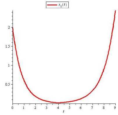
Fig.1 The graph of approximated х_г ( t )

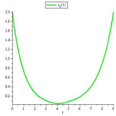
Fig.2 The graph of approximated Х₂ ( t )

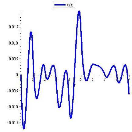
Fig.3 The graph of approximated control

Example IV.2 Consider the following optimal control problem (see[14]):

1min I =  ((x^(2)-4)2+(X2(2) -2)2)

1+  ∫((X2 (t)-2) +u2 (t)) dt

s․t․ ̇(t)=0-0․․8  3․․41x(t)+⌊1⌋и(t),0≤t≤К,̇(t)=04   31X(t)+⌊2⌋и(t), 14 ≤t≤2,X(0)=⌊Xl (0)  ^2 (0)⌋ T=⌊0  2⌋T․

Let к =20 and,n=3․ By using mentioned algorithm, we found that the switched instant is Ti = 0․17, and the approximated objective function by this method is 9․329921749. From (17), one can find the following solution.

Xi ( t )=

• -10․92427311 t - 88․99616160 t² + 825․9280790 t³

• ^⎧  1․915913401 - 68․06241582 + 478․9926727t² - 1056․059394t³

• ^⎪ -3․229687448 + 34․57688896 - 161․4803114 t² + 223․5230136 t³

• ⎪  1․109324474 - 18․25900824 + 46․12527240t² - 42․13422000 t³

⎪-0․6947052100 - 2․099877390 - 0․8448252000t2 + 2․484420000t3

⎪ -0․5021273950 - 3․867739620 t + 3․915690000t² - 1․505784000t³

⎪ -0․5161999930 - 3․694819410 t + 3․456561000t² - 1․155752000t^{3 ⎪}-0․8579139600 - 2․237479440 t + 1․384858800t² - 0․1740900000t³

⎪-1․069491944 - 1․448535120 t + 0․4042698000t² + 0․2321590000t³

-1․540205516 + 0․1226180700 t - 1․343798100t² + 0․8804590000t³

-2․227859986 + 2․183996040 t - 3․403590600 t² + 1․566528000t³

⎪  -3․388089573 + 5․347624890 t - 6․279040800 t² + 2․437702000 t³

⎪ -5․335317045 + 10․21424673 t - 10․33335330 t² + 3․563565000 t³

⎪  -8․629786951 + 17․81489547 t - 16․17848760t² + 5․061928000t³

^⎪  -14․17822747 + 29․70144651 t - 24․66676380 t² + 7․082442000t³

⎪  -23․43852405 + 48․21801782 t - 37․00846345 t² + 9․824446100t³

⎪ -38․78543661 + 76․98657422 t - 54․98449581 t² + 13․56855380t³

⎪ -63․72782578 + 120․9970447 t - 80․86976648 t² + 18․64346150t³

⎪ -104․8969032 + 189․5942580 t - 118․9693762 t² + 25․69710160t³

⎩ -166․8730805 + 287․4592285 t - 170․4813861 t² + 34․73502100 t³

0≤ t ≤ 0․1, 0․1≤ t ≤ 0․2, 0․2≤ t ≤ 0․3, 0․3≤ t ≤ 0․4, 0․4≤ t ≤ 0․5, 0․5≤ t ≤ 0․6, 0․6≤ t ≤ 0․7, 0․7≤ t ≤ 0․8, 0․8≤ t ≤ 0․9,

0․9≤ t ≤1, 1≤ t ≤ 1․1, 1․1≤ t ≤ 1․2, 1․2≤ t ≤ 1․3, 1․3≤ t ≤ 1․4, 1․4≤ t ≤ 1․5, 1․5≤ t ≤ 1․6, 1․6≤ t ≤ 1․7, 1․7≤ t ≤ 1․8, 1․8≤ t ≤ 1․9,

1․9≤ t ≤2,

2․- 6․247657080 t - 119․6884392 t² + 1084․037550t³          0≤ t ≤ 0․1,

-0․3984525320 + 36․49191078 t - 254․9440368 t² + 561․0892720t³

2․171670672 - 15․87093006 t + 75․92513130 t² - 105․4509480t³ 0․08271634800 + 9․535033560 t - 23․81614860 t² + 22․10017900 t³

х₂ ( t )=

⎪ 1․001349292 + 1․266263400 t + 0․3033345000 t²

⎪ 0․9188825670 + 2․055907800 t - 1․865642400 t²

⎪ 0․9193868190 + 1․999410480 t - 1․681520100 t²

^⎪ 1․074010659 + 1․339149300 t - 0․7417362000 t²

⎪ 1․144599331 + 1․075936500 t - 0․4145886000 t² 1․313990014 + 0․5091870600 t + 0․2174817000 t² 1․539067314 - 0․1667255400 t + 0․8940750000 t²

⎪ 1․911500265 - 1․184286840 t + 1․820799000 t²

⎪ 2․529563493 - 2․731854810 t + 3․112447200 t²

⎪  3․578206933 - 5․155375620 t + 4․979443500 t²

^⎪  5․358414131 - 8․975245350 t + 7․711593300 t²

8․357182676 - 14․98034238 t + 11․72003130 t²

⎪  13․38164245 - 24․41145534 t + 17․62088370 t²

⎪  21․60103076 - 38․93241147 t + 26․17212450 t²

⎪ 35․49431179 - 62․10123567 t + 39․05111340 t²

⎩ 56․59052004 - 95․41579482 t + 56․58759540 t²

- 0․8723550000t3

+ 0․9667550000t3

+ 0․8144870000t3

+ 0․3686120000t3

+ 0․2330790000t3

- 0․001891000000t3

- 0․2276490000t3

- 0․5089800000t3

- 0․8683290000t3

• -    1․347751000t³

• -    1․999137000t³

  - 2․891021000t³

• -    4․121700000t³

• -    5․800277000t³

• -    8․186649000 t³

• -    11․26366400 t³

0․1≤ t ≤ 0․2, 0․2≤ t ≤ 0․3, 0․3≤ t ≤ 0․4, 0․4≤ t ≤ 0․5, 0․5≤ t ≤ 0․6, 0․6≤ t ≤ 0․7, 0․7≤ t ≤ 0․8, 0․8≤ t ≤ 0․9,

0․9≤ t ≤1, 1≤ t ≤ 1․1, 1․1≤ t ≤ 1․2, 1․2≤ t ≤ 1․3, 1․3≤ t ≤ 1․4, 1․4≤ t ≤ 1․5, 1․5≤ t ≤ 1․6, 1․6≤ t ≤ 1․7, 1․7≤ t ≤ 1․8, 1․8≤ t ≤ 1․9,

1․9≤ t ≤2,

and,

-12․- 271․9368459 t + 4813․469301 t² - 12235․54335t³          0≤ t ≤ 0․1,

и ( t )=

-107․3673603 + 1966․962301 t - 11354․30555 t²

^⎪  103․1832786 - 1187․617197 t + 4400․191513 t²

-62․01583519 + 497․3348902 t - 1326․185276 t²

20․06701776 - 137․4718584 t + 308․7949736 t²

-8․365959965 + 41․83694681 t - 67․24451456 t²

-0․9632493676 + 2․764604054 t + 1․307372980 t²

⎪ -0․7599670345 + 3․225506185 t - 1․254075950 t²

⎪-0․4567610441 + 2․548305161 t - 0․9823514700 t²

1․252018664 - 2․353197923 t + 3․581063870 t²

2․995233768 - 6․617740527 t + 6․880503770 t²

⎪   6․141198540 - 13․87490271 t + 12․27543144 t²

⎪   11․09308293 - 24․38528583 t + 19․47631084 t²

⎪   19․22373651 - 40․45418733 t + 29․76458490 t²

⎪   32․45124930 - 64․88261913 t + 44․41615156 t²

⎪   54․02509013 - 102․3256824 t + 65․57511486 t²

⎪   88․27499645 - 158․2371555 t + 95․32784724 t²

⎪   144․8752853 - 246․1052081 t + 139․9474017 t²

⎪   229․3779020 - 369․2999893 t + 198․5873282 t²

⎩  364․6997357 - 559․1462311 t + 285․9696600 t²

+ 20919․65079 t³

- 5307․176954 t³

+ 1177․541515 t³

- 224․9115092t3

+ 37․39606800 t³

- 2․594600800 t³

- 0․4686645000 t³

- 0․3423927000 t

- 1․705620900t3

- 2․483733300 t³

- 3․754168200t3

- 5․321697700t3

- 7․428327100 t³

- 10․25076840 t³

- 14․10763160 t³

- 19․22446370 t³

- 26․58760470 t³

• -    35․63173580 t³

• -    48․76254090 t³

0․1≤ t ≤ 0․2, 0․2≤ t ≤ 0․3, 0․3≤ t ≤ 0․4, 0․4≤ t ≤ 0․5, 0․5≤ t ≤ 0․6, 0․6≤ t ≤ 0․7, 0․7≤ t ≤ 0․8, 0․8≤ t ≤ 0․9,

0․9≤ t ≤1,

1≤ t ≤ 1․1,

1․1≤ t ≤ 1․2, 1․2≤ t ≤ 1․3, 1․3≤ t ≤ 1․4, 1․4≤ t ≤ 1․5, 1․5≤ t ≤ 1․6, 1․6≤ t ≤ 1․7, 1․7≤ t ≤ 1․8, 1․8≤ t ≤ 1․9,

1․9≤ t ≤2․

The graphs of approximated trajectories, and approximated control are shown respectively in Figures 4 and 5.

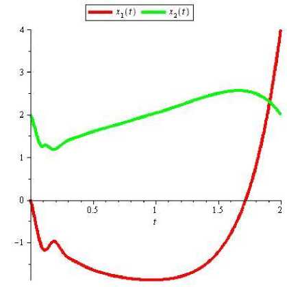
Fig.4 The graphs of approximated trajectories

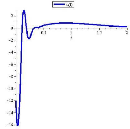
Fig.5 The graph of approximated control

V. Conclusions

In this paper, we studied optimal control problems for switched systems in which a pre-specified sequence of

active subsystems is given. Based on Bezier control points, we proposed a method to obtain the approximated trajectories and control. This note first transcribes an optimal control problem in to an equivalent problem parameterized by the switching instants and then uses the Bezier control points method. The original new problem is converted into a nonlinear programming problem (NLP) by applying Bezier control points method, whereas the MATLAB optimization routine FMINCON is used for solving resulting NLP. Numerical example shows that the proposed method is efficient and very easy to use.