Optimal Power Flow Solution using Efficient Sine Cosine Optimization Algorithm

Published Online April 2020 in MECS

Nowadays, optimal power flow (OPF) is an essential field in modern power systems market and investment. The major goal of the optimal power flow is to reduce some types of objective functions under conditions that are some constraints are respected, in order to determine the set of setting variables in the power network. The equality constraint is the equilibrium state of power systems represented by power flow equations to check the equality between the generation and the demand. The feasible range of all variables to ensure security and operation conditions which represent the inequality constraints. The variables which are changed in the optimization process to give the optimal solution are called the variables of control. The active generator powers in generating bus except in slack bus (PV buses), voltage amplitudes in generating unit, transformer regulating ratios and reactive power of shuntcompensator are cited among the set of variables of control.

Whereas, the states variables are found by the state of power systems and are depend on variables of control among them we listed the active generator power of slack bus, amplitude voltages in load bus (PQ buses), the phase angles in PV and PQ buses, the generator reactive powers, and the apparent power flow in transmission line. Consequently, the combination of the constraints and all variables with certain objectives function the OPF problem convert to the non-smooth, non-convex and nonlinear optimization problem.

After the modeling of the optimal power flow problem, the optimization of the OPF becomes easy by applying appropriate methods. For this, there are classical methods and metaheuristic methods. Various classical algorithms are applied to solve the problem of the optimal power flow (OPF). These algorithms include traditional linear and nonlinear methods. Nonlinear methods include: reduced gradient method, Newton method, successive quadratic method and interior point method which is the newest and the most effective method. All these methods are based on Lagrange formulation and the condition of Kurush and Kuhn-Tucker[1-4]. Although, they are precise and fast but require several calculations and converge almost to the local optima for non-convex cost function. Recently, standard meta-heuristic methods are used in the OPF problem based on stochastic intelligence techniques of agents in the group, which are applied for the global solution. The most important methods are the genetic algorithm (GA) and improved GA [4-8], evolutionary programming (EP) [9], improved evolutionary programming (IEP) [10]. Additionally, The application of particle swarm method (PSO) [11], parallel processing with PSO (PPPSO) and differential evolution (DE)[13] are used to solve large OPF problem. Novel meta-heuristic methods inspired by physical laws and behavior of animals and insects in nature are widely used for solving the OPF problem. Among them they are shuffled frog leaping algorithm (SFLA) [14],gravitational search algorithm (GSA)[15,16], biogeography-based optimization (BBO)[17], harmony search algorithm (HS) and improved harmony search algorithm (IHS)[18-20], artificial bee colony algorithm (ABC) [21],differential search algorithm (DSA)[22,23], teaching-learning-based optimization technique (TLBO)[24], krill herd algorithm (KHA)[25], improved electromagnetism-like mechanism method (IELM)[26], improved colliding bodies optimization algorithm(ICBO)[27], black-hole-based optimization (BHBO)[28], Firefly algorithm[29], Grey Wolf Optimizer (GWO) [30], Jaya Algorithm (JA) [31], moth swarm algorithm (MSA)[32] and Enhanced Flower Pollination Algorithm (EFPA)[33].

Most of these methods are applied to solve the OPF problem with convex, non-convex, non-smooth cost functions and other objectives such as voltage profile improved and voltage stability enhancement. They exist other improved methods to enhance the convergence and solution such as oppositional and quasi-oppositional biogeography-based optimization (OBBO, QOBBO)[34,35], quasi-oppositional Jaya algorithm (QOJA) [36], the combination of the particle swarm and gravitational search method (PSOGSA) developed in [37]. Also, the combination of Differential evolution and Harmony search algorithm (DEHS) [38]. In [39] a differential evolution algorithm integrated with different handling techniques with self-adaptive penalty (SP) as the better and an ensemble of the constraint handling are used to improve the solution of the multi-objective optimal power flow.

The main problem encountered in the meta-heuristic algorithms is the convergence to the worst global optima, thus it is due to the worst choice of the appropriate setting parameters. In the present paper, an efficient sine cosine algorithm (ESCA) is applied to solve the optimal power flow problem. The sine-cosine algorithm (SCA) is a novel meta-heuristic method uses sine and cosine formulation for each generation to reach the optimal solution, first was developed and detailed by Mirjalili [40]. In [41] a sine-cosine algorithm and modified sine cosine with levy flights are added to the original sinecosine algorithm have been detailed for optimizing the multi-objective OPF to enhance the convergence to the global optimum. But, the improved SCA is difficult compared to the standard SCA method, which is a simple and works with few parameters with simple formulation of updating the position of individuals in the group. In this paper, the appropriate parameters of (SCA) are chosen to improve the quality of the solution and accelerate the convergence to the best global optimum.

Various types of objective functions have been optimized by ESCA method on standard IEEE 30bus. In order to validate the results, a discussion and a comparison have been achieved with other meta-heuristic methods. Consequently, this technique improves greatly the quality of the solution and the rapidity of the convergence.

The organization of this paper is detailed as flow: an introduction in section I. Problem Formulation with different types of objective function of optimal power flow is modeled in section II. The details of SCA and ESCA with modified parameters are given in section III.

In section IV a numerical results with comparison are discussed in section V. Finally, a conclusion is showed for evaluating this work.

• II.    Problem Formulation

By the combination of different objective and constraint with all variables the OPF problem can take the following form:

Minimize F(s, u)(1)

subject to G(s, u)(2)

and H(5,u) < 0(3)

Where F(s,u) is the objective function, G(s,u) is the equality and H(s,u) is the inequality constraints. S is the vector of state variables and U is the vector of control variables, the two vectors are given by:

S = ⁽ Pg    , 2 ,..' П n , V I i ’-V L^    Q g _x ,Q gn_e , S L i ,", S L nbr ) ⁽⁴⁾

Where P gslack is the slack active generator power, 0 the angle of PV and PQ buses, V_L the amplitude voltages of PQ buses, Q _g the reactive powers in generator and the S_L is the apparent power in transmission lines.

We denote by P _g : the active powers in PV buses, V _g : the amplitude voltages of generators, T : the regulating transformers ratios and Q_c reactive power of shunt compensators.

The number of buses, the number of PQ buses, the number of generators, the number of tap transformers, the number of shunt compensators and the number of lines are denoted by n,nl, ng, nt ,nc , nbr respectively .

• A.    Objective Function Types

Many objectives functions are studied to ensure the goal of the optimal power flow problem. Most of the objective functions are detailed in the next section:

• a.    Production Fuel Cost

The main objective function in the OPF problem is the total production cost caused by the fuel used in the unit of generation:

ng

F c = £ C i (P)

i = 1

NL

F v = F + ® v £ V - 1

i = 1

Where C i : is the production cost of thermal unit n i given in simple convex and smooth quadratic model which is given by:

C i ( P gi ) = a i + b i P gi + cP (7)

Where: P gi is the generator active power at unit i and a i , b i and c i are the cost coefficients of i^th unit.

For multi quadratic model, the fuel cost takes multi function for each interval of generating power which explained by using of multiple fuel form the unit. The problem for this type becomes a non-convex optimization problem. The production cost in (6) is expressed by the following model:

	a i1	+ b i1 P gi + C i 1 Pgi	if	min gi       gi     gi 1
C i ( P gi ) =	ai 2 ...	+ b ,2 P gi + C i 2 P g 2	if	P .. < P . < P ...           zox J gi 1 -i gi -i gi 2             (8)
	. a im	2 im gi    im gi	if	max gi ( m - 1) - gi - gi

Where: a im ,b im and c im are the cost coefficients of fuel type m in the i^th unit.

To increase the efficiency of generating unit a number of admission valves are added and switched successively causing fluctuation form in the function. The effect of these valves is appeared by addition of sine component in the cost function; therefore this model converts to the non-smooth cost function. Then the model of cost with the effects of valves is given by the equation:

C i ( P gi ) = a i + b i P gi + c . P ² + | e i x sin( f_t(P gi min - P gi )|    (9)

Where: e i and f i the coefficients of the sine components of the valves.

• b.    Active Power Loss

The minimization of the total active power loss in the power network is essential which caused by the bad effect of the reactive power circulation. Consequently, the total active power loss can be formulated as follows:

F l = £ g k (V ² + V j - 2-- cos e j )     (10)

k e Nbr

Where g k : is the real part of admittance of the line (i-j), n br : is the total number of electric lines in power systems.

• c.    Voltage Deviation Improvement

Sometimes, it is desirable that the voltage should be close to a nominal value (1p.u.), which is reflected by the reduction of the voltage amplitude deviation at load buses. Then the objectives function for both the fuel cost and the voltage deviation convert to:

• d.    Voltage Stability Enhancement

The improvement of the voltage stability is achieved by minimizing the stability index L of load buses. This objective is attained by minimizing the global maximum index L max :

Lmax = max {Lk } , k e npq

We define the index Lk of load bus k:

L k =

1 + Vk-V k

V ok : is the voltage of bus without load:

Ng

V =-V H V(14)

ok2

i = 1

H 2 is a matrix defined by partial inversion of admittance matrix of orderly Y bus to PQ, PV buses, and then we have:

h 2 =- y;Y             (15)

Finally, the objective function of this problem is formulated by:

F = F + ^ L^          (16)

SL max

Where: ω L is a weighting factor of voltage stability.

• B.    Equality Constraint

The equality constraint describes the equilibrium state of the system during the optimization process. It can resolve by Newton Raphson load flow equation to find all state variables. These variables confirmed the balance equation which is the production power equal the demand power plus losses.

n g

£ P gi = P d + P L              ⁽¹⁷⁾

i = 1

• C.    Inequality Constraints

To ensure the good operation of equipment in the power system, it must keep certain variables in their limits which are represented by h(s,u). Among them we list the generated active and reactive powers; the bus voltage magnitudes of all buses, the transformers tap settings and the compensators reactive powers:

P„__

gi min      gi     gi max ,       g

О ™ < О < О ™ Jen gimin      gi     gimax ,      g

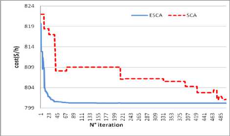
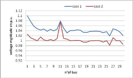
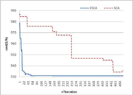
V--

Ti min < Ti^ Ti    i e nt

Line power flow constraints: the constraint of transmission lines loading is given by:

Sl,< Sm^x, i e nbr               (19)

• D.    Global Objective function

In meta-heuristic search algorithms, all control variables remain within their limits except the slack bus active power. We add the inequality constraints related to the state variables to the objective function by multiplying with penalty factors. Therefore, the augmented or fitness function form of the objective function becomes:

nl

FT = F + kp(P -P .)2 + kv2(V - V, i=1

ⁿg                                 nbr

+kq 2 (Qgi- Qgm)2 + ks 2 (Sli- SD2 i=1

xk⁺¹

Where: kp ,kv ,kq and ks are the penalty factors P_g^li_s^m_lack Vi^limand Q_g^lim are defined as:

lim       minmin

1 gslack 1 gslack lvr 1 gslack < 1 gslack lim       maxmax pgslack  pgslack for Pgslack > pgslack

<

V^llm= Vmin for V< V

Vlug = VimaxforVi > V min

max

Qgirn = Qmn foQ< Qmn

Q' = Qmax NQ_g> Q_gmax g  g   gg

F is the total cost function given by (6), real power losses given by (10), cost with voltage profile given by (11), or F of total cost with voltage stability is given by (16).

The equality constraint is solved by Newton-Raphson load flow equation.

• III.    Sine-Cosine Optimization Method

Sine Cosine Optimization Algorithm (SCA) is a global optimization Algorithm was introduced and detailed by Mirjalili [40]. Its principle process consists of searching stochastically the best vector of control variables from an initial group of members and converges to the best solution in the search space or diverges from it in fluctuating manner, using a simple mathematical formulation based on sine and cosine functions.

Compared to other methods, the SCA method has a few control parameters and easy to implement. Whereas SCA works on a group in which the members move by changing their positions and converge to the optimal solution in the feasible domain. The number of members in the group is np and the initial population of the SCA is randomly generated within the feasible ranges of control variables. Each member adjusts its position to the best destination using sine and cosine formulation. In the SCA a member is represented by the vector Xi = Xij ,i enp,jend which their elements represent the variables of control. The reverse operation for calculating the objective function and determining the elements of control variables we put Uj = Xi,j,i e n_p; j e n_d. In the optimization process, the destination Xgbest = C^^gbest,....x^gb^est; represents the best member which has the best fitness function among all the members in the group. The updated position of member n°i modified under the following equation:

xk + r1 xsin(r₂)x |r₃Xgbestk -xi^k|; r₄^ 0.5

xk + r1 x cos(r₂) x r₃Xgbestk - xk ; r₄ > 0.5

Where: x_i^K : is the position of the current solution at k^th iteration, r2,r3,r4 are random parameters in the range of [0,2^] ,[0,2] [0,1] respectively.

Xgbest^k : The best position or destination of the group until iteration k.

r1 is an iterative adaptation parameter (conversion parameter) decreases from a to 0 with the number of iteration increase from 0 to kmax and was given by the following expression:

Where a: is a constant parameter and kmax is the maximum number of iterations.

The parameter r1 describes the movement of the individual in the next position. Thus if r1 <1 the updated individual is situated in the region between the previous position and the best vector (destination) else the updating vector is situated outside.

The parameter r2 is designed to measure the distance of movement of convergence or divergence to the destination.

The parameter r3 is a weighting factor to adjust the destination, rather than it is an important parameter and defines the speed of convergence and the quality of the solution to the best agent.

The parameter r4 is the random value which its role is to change the use of sine or cosine component such as in equation (22).

• A.    Efficient SCA

To improve the SCA algorithm for the best global solution with speed convergence, it should to choose the appropriate parameters of the SCA algorithm. In standard SCA the control parameters r2 and r3 take the value r2 = 2* n *rand[0,1]and r3 = 2*rand[0,1] respectively.

Where rand [0,1] is a random number in range [0, 1], r1 is given by equation (23). In the efficient ESCA the optimal parameters are modified as follow:

The parameter r₁ take random value in interval [0, 2] then we set r₁=2*rand[0,1], r₃ take a constant value which equal to r3=1 to accelerate the convergence, r2 is not changed. The steps of the algorithm are listed in the following section.

• B.    Algorithm of ESCA and SCA

ESCA and SCA have the same steps of the algorithm; the difference appears in the choice of setting parameters. The main steps of ESCA and SCA algorithms are detailed as follow:

• 1-    Initialize randomly np vectors between the limits of control variables U by the following expression:

x⁰. = umin + rand * (u^max- u^m^)          (24)

Where ien_P,jend and um^ax,u^minare lower and upper limits of control variables respectively. Rand is a random number in interval of [0, 1].

• 2-    Set Xi = Xi⁰and the iteration counter to k=1.

• 3-    The fitness function of all elements Xi are determined using global function F (eq. 20) and select the destination Xgbest the best element which has the best value among elements X, where i e n_P

• 4-    Update the parameters: rj, r₂, r₃, r₄ for each element of ^Xi

• 5-    Change the position of the actual member Xi using SCA updating equation (22), and determine the new elements X_i

• 6-    Check the test limits, if the elements of Xi violate the upper or lower bound of control variables; it must take this upper or lower bound.

• 7-    If k < k_max set k=k+1 and go to step 3 otherwise go to step 8.

• 8-    Take Uc^pt = Xgbest and run load flow to calculate real slack power, other elements of state variables, fuel cost and active power losses.

For evaluating the global function for each iteration, it must solve the power flow equation which is the equality constraint. After that all state variables, active power losses are found and the process of optimization is continued.

• IV.    Numerical Results and Discussions

In order to validate the application of the ESCA compared to SCA algorithm, we consider the standard IEEE 30-bus with 41 branch systems [2] for minimizing various functions. The dimension of the vector of control variables is nd =24 which includes 5 generator-bus active power, 6 generator-bus voltage magnitudes, 4 transformer-tap settings, and 9 bus shunt reactive compensators. The bus n°1 is chosen as the slack bus, 2, 5, 8, 11 and 13 are chosen as PV buses and the rest are PQ (load) buses. The cost and active power loss of initial load flow base case are 901.8 $/h and 5.8 MW respectively.

The permissible ranges of transformer tap settings are 0.9p.u and 1.1 p.u respectively, the permissible ranges of generator bus voltage are 0.95 p.u and 1.1 p.u respectively, and the permissible ranges of load bus(PQ buses) voltage are 0.95p.u and 1.05 p.u respectively. The permissible ranges of reactive power of shunt compensators are 0 p.u and 0.05 p.u. The coefficients of the fuel cost functions and the permissible ranges of the real power of generators are given in table 1.

Table 1.Generators Cost coefficients and generators active power limits

	Real Power output Limit(MW)		Cost coefficients
Bus N°	Min.	Max.	a($/h)	b( $/MWh)	c($/(Mw)2h)
1	50	200	0	2.00	0.00375
2	20	80	0	1.75	0.01750
5	15	50	0	1.00	0.06250
8	10	35	0	3.25	0.00834
11	10	30	0	3.00	0.02500
13	12	40	0	3.00	0.02500

The population size in ESCA and SCA is equal to 50. For each problem types, we choose kmax=500 which is the maximum number of iterations. The constant parameter a in equation (23) of r₁ is a=1.5 for standard SCA algorithm.

Table 2 and table 5 show the OPF results obtained by the proposed ESCA method for various types of functions. Simple fuel cost, fuel cost with voltage profile improvement, fuel cost with voltage stability and total real power losses are minimized by ESCA and SCA. Also, other types of non-convex and non-smooth fuel cost are optimized such as the cost with the different type of fuels and fuel cost with valves effects.

To obtain the best global optimum several executions of the ESCA method have been achieved for each type of functions. The results listed in table 2 and table 5 is the best solution of the ESCA method.

• A.    Type1: Simple Production Cost Function

  The first simulated type of optimization is the minimization of simple quadratic fuel function which is given by equation (6) and introduced in augmented objective function given by equation (20) to respect all constraints. The results obtained by ESCA are listed in type 1 of table 2 of which give the fuel cost of 800.2198 $/h with the voltage deviation of Vd=0.9454 p.u. The characteristic of convergence of ESCA compared to the SCA is shown in figure 1. From the results and figure of convergence of simple fuel cost function which is a convex function, it is clear that the ESCA is converged

fast than SCA to the best global optimum. The inequality constraints of all variables are respected and all variables remained in their permissible ranges.

Fig.1. Convergence characteristics of SCA and ESCA algorithms of Type 1.

Table 2. Simulation results with ESCA of types 1,2 and 3.

Control variables	Type 1	Type 2	Type3
Pg1(MW)	177.6493	177.1922	177.1127
Pg2(MW)	48.6658	49.3761	48.8634
Pg5(MW)	21.3344	21.8592	21.3803
Pg8(MW)	20.9348	23.2242	21.2303
Pg11(MW)	11.8018	10.0000	11.8190
Pg13(MW)	12.0000	12.0000	12.0000
V1(pu)	1.1000	1.0254	1.0867
V2(pu)	1.0767	1.0113	1.0681
V5(pu)	1.0430	1.0146	1.0389
V8(pu)	1.0457	1.0051	1.0460
V11(pu)	1.0788	1.0745	1.0630
V13(pu)	1.0313	1.006	1.0569
T4,12	0.9456	0.9688	0.9922
T6,9	1.0603	1.1000	0.9720
T6,10	0.9332	0.9000	1.1000
T28,27	0.9809	0.9718	0.9682
Q10 (pu)	0.0500	0.0500	0.05
Q12(pu)	0.0000	0.0000	0.05
Q15(pu)	0.0500	0.0500	0.05
Q17(pu)	0.0500	0.0000	0.05
Q20(pu)	0.0413	0.0500	0.05
Q21(pu)	0.0500	0.0500	0.05
Q23(pu)	0.0304	0.0500	0.05
Q24(pu)	0.0500	0.0500	0.05
Q29(pu)	0.0258	0.0277	0.05
Cost ($/h)	800.2198	804.9968	800.4102
Active Losses (MW)	8.9861	10.2517	9.0057
Vd(pu)	0.9454	0.09163	0.9774
Lmax	0.1267	0.1367	0.1224

The results of proposed ESCA are compared only with other solutions reported in the literature. The comparison of results is shown in Table 3.

ESCA gives a good global minimum compared to other meta-heuristic methods reported in the literature such as (JA)[31], Moth swarm algorithm (MSA)[32], superiority of feasibly solutions differential evolution (SF-DE) [39], sine cosine algorithm (SCA)[41], modified SCA (MSCA) [41]which give 800.41 $/hr, 800.660 $/h, 800.3887$/h, 801.410$/h, 800.4985$/h, 800.4794$/h, 800.5099$/hr, 800.4131$/hr, 800.1020$/hr, 799.3100 $/hr respectively.

It is observed that ESCA gives the best value of cost than other methods with an acceptable value of Vd. SCA[41] MSCA[41] give a minimum values than ESCA with the important values of Vd which are 2.0825 p.u and 1.4246 p.u. respectively. The important value of Vd represents the most violations of voltage limits in load (PQ) buses which is infeasible solution.

• B.    Type 2: Cost with Voltage Profile

  In type 2, both the fuel cost and voltage profile are considered for the minimization, for the reason to improve the quality of service by reduced voltage margin. This type of function is given by equation (11) and (20). The results after the optimization of all control variables and functions are listed in table 2 type 2 of ESCA results. The production cost provided by the proposed ESCA is 804.9968 $/h with voltage deviation Vd=0.09163 p.u.

It is clear that the voltage deviation of PQ buses Vd is greatly improved by using ESCA than SCA[41], MSCA[41] which give 0.1082 p.u. and 0.1030 p.u. respectively.

We observe that the voltage deviation Vd obtained in case 2 is reduced than the Vd obtained from case 1. Diagram of voltage amplitudes for all buses of type 1 compared to type 2 obtained by ESCA is illustrated in Figure 2. It is clear that the voltage magnitudes in PQ buses approach to 1 p.u. of case 2.

For the comparison with other methods such as: PSO[11], DSA [23]; GWO[30], PSOGSA[37], JA [31], MSA[32], (SF-DE) [39] which give respectively : 0.0891p.u, 0.13570 p.u, 0.09700 p.u, 0.09638 p.u, 0.10842 p.u, 0.09454 p.u . It is observed that ESCA gives a better value of Vd with acceptable total cost than these previous methods.

Fig.2. Diagram of voltage magnitudes of Type 1 and Type 2 of ESCA algorithm.

• C.    Type 3: Cost with Voltage Stability

  We added the voltage stability index to the simple quadratic cost function for increasing the performance of the system, which is considered in this case (such as in equation 16). After the application of ESCA we obtain the optimal values of control variables as given in type 3 of Table 2. Thus, the maximum voltage stability index Lmax is reduced by ESCA from 0.1267 to 0.1224 and the cost increases to 800.4102 $/h, also V_d increases to

  0.9774p.u. All inequality constraints are respected, the most important is the voltage limits which are represented by good value of voltage deviation Vd It is observed that ESCA gives the best solution than other methods cited in references such as ABC[21], DSA[23], PSOGSA[37], JA[31], MSA[32], SF-DE[39] which give respectively 0.13790 p.u , 0.12499 p.u , 0.12393 p.u , 0.12430 p.u , 0.13713p.u, 0.13745 p.u. The comparison of different results shows that ESCA method improves greatly the solution with the good total cost with minimum Lmax.

Table 3. Comparison results of different methods for type 1 and 2

Methods	Type n°1		Type n°2
	cost	Vd	cost	Vd
PSO [11]	800.41	0.8765	806.38	0.0891
ABC[21]	800.660	/	/	/
DSA [23]	800.3887	/	805.261	0.1357
6GWO[30]	801.410	/	803.631	0.0970
PSOGSA[37]	800.4985	0.91373	804.431	0.0963
JA[31]	800.4794	/	/	/
MSA[32]	800.5099	0.9035	803.312	0.1084
SF-DE [39]	800.4131	0.9209	803.719	0.0945
SCA[41]	800.1020	2.0825	843.604	0.1082
MSCA[41]	799.3100	1.4246	849.281	0.1030
ESCA	800.2198	0.9454	804.99	0.0916

Table 4. Comparison results of different methods for type 3 and 4

Methods	Type n °3		Type n°4
	cost	Lmax	Ploss	Vd
PSO [11]	/	/		/
ABC[21]	801.6650	0.13790	3.10780	/
DSA [23]	800.9331	0.12499	3.09450	/
َ6GWO[30]	/	/	3.41	/
PSOGSA[37]	801.2292	0.12393	/	/
JA[31]	840.7181	0.12430	3.1035	/
MSA[32]	801.2248	0.13713	3.1005	0.88868
SF-DE [39]	800.4203	0.13745	3.0844	0.90359
SCA[41]	/	/	2.9425	1.8161
MSCA[41]	/	/	2.9334	1.5987
ESCA	800.4108	0.1224	3.0212	1.1317

D. Type 5: Real power losses minimization

The minimization of real power losses is treated in this case like as in equation (10) and total function (20). Real power losses are reduced by ESCA to 3.0212 MW with Vd of 1.1317 p.u, see table 5 type 4. It is clear that the total active power losses are greatly reduced from the initial value of the load flow base case which is 5.81 MW. For the comparison with other methods listed in references, the ABC[21], DSA[23] , GWO[30], JA[31], MSA[32], and SF-DE[39] give 3.1078 MW, 3.0945, MW 3.41 MW, 3.1035 MW, 3.1005 MW, 3.0844 MW, respectively. SCA[41] and MSCA[41] give 2.9425 MW and 2.9434 MW but it is an infeasible solution represented by the high value of Vd which caused by most violations in voltage amplitudes limits of PQ buses. It is observed that ESCA gives a good minimum of active power losses with acceptable V_d than the other methods.

• E.    Type 5: Multi fuel Cost Model

For this type of non-convex function, the cost takes multiple quadratic forms in each range of real generators power according to the equation given by (8). This model of the cost function is introduced in the generators buses n°1 and n°2 and represented by piecewise quadratic functions which the cost coefficients are given in [11].

In this type, the results of the ESCA is given in Table 5 type 5, the cost obtained by ESCA is 646.4095 $/hr, with Vd of 0.9645 p.u, therefore SCA[41] and MSCA[41] give 648.1366 $/hr and 646.3600$/hr respectively.

For this type of function, ESCA gives a better result compared to the SCA method and almost the same result as the MSCA method. Also, all limits on control and state variables are respected.

For proving the speed convergence of the ESCA method of a non-convex cost function, the characteristic of convergence is illustrated in figure 3. We observe that ESCA with new parameters converges fast with high robustness and stability to the best value than SCA.

From the results it can be concluded that ESCA is able to solve the optimization problems with non convex function with high convergence stability.

Table 5. Simulation results with ESCA of types 4,5 and 6.

Control variables	Type 4	Type5	Type6
Pg1(MW)	51.4212	139.9998	196.9976
Pg2(MW)	80.000	54.9994	52.057
Pg5(MW)	50.000	24.2163	15
Pg8(MW)	35.000	35.0000	10
Pg11(MW)	30.000	19.7111	10
Pg13(MW)	40.000	16.1524	12
V1(pu)	1.0768	1.0874	1.0389
V2(pu)	1.0723	1.0719	1.0152
V5(pu)	1.0527	1.0432	0.95
V8(pu)	1.0586	1.0516	1.0256
V11(pu)	1.0634	1.1	1.0518
V13(pu)	1.0627	1.0495	1.0534
T4,12	0.9967	0.982	1.1000
T6,9	1.0823	1.1	1.1000
T6,10	0.9000	0.9	1.1000
T28,27	0.9838	0.9851	1.0021
Q10 (pu)	0.0500	0.05	0.0500
Q12(pu)	0.0500	0.05	0.0500
Q15(pu)	0.0500	0.05	0.0000
Q17(pu)	0.0500	0.00	0.0000
Q20(pu)	0.0500	0.05	0.0500
Q21(pu)	0.0500	0.05	0.0500
Q23(pu)	0.0295	0.00	0.0500
Q24(pu)	0.0500	0.00	0.0500
Q29(pu)	0.0226	0.05	0.0000
Cost ($/h)	967.6184	646.4095	930.9864
Active Losses	3.0212	6.6790	12.6546
(MW)
Vd(pu)	1.1317	0.9645	0.70831
Lmax	0.1271	0.1266	0.1188

Fig.3. Convergence characteristics of SCA and ESCA algorithms of Type 5

Compared to the improved colliding bodies optimization algorithm (ICBO)[27], MSA[32], SF-DE [39],SCA[41], MSCA[41] which give respectively: 645.1668 $/h646.8364$/h, 646.4390$/h, 648.1366$/h and 646.3600 $/h, it is observed that ESCA method gives a good minimum cost with feasible solution of voltage constraints. Really ICBO[27] gives the better solution but is not a feasible solution represented by the high value of Vd which is 1.8232 p.u caused by the violation of voltage limits.

• F.    Type 6: Production Cost Functions with Admission Valve Effects

  The effect of valves is added to generator buses No. 1 and No. 2; the coefficients of the cost are given in [11]. Thus the expression of the cost was given by the equation (9), and introduction in the global form such in equation (20). Also, the minimum cost obtained by ESCA is 930.9864 $ /h, with 0.7083 p.u. of Vd as given in table 5 type 6. But SCA with old parameters gives 935.699$/h with V_d as 0.9589 p.u. Obviously that ESCA gives a better solution than SCA with best Vd to restrict the violations in voltage limit constraints.

It is obvious that ESCA converges fast to the better solution than SCA. The characteristic of convergence is illustrated in figure 4 and show the fast convergence to the global solution of non smooth function type.

Table 6. Comparison results of different methods

Methods	Case n°5		Case n°6
	cost	Vd	cost	Vd
ABC[21]	/	/	931.7450	0.4575
ICBO[27]	645.1668	1.8232	/	/
MSA[32]	646.8364	0.84479	930.7441	0.44929
SF-DE [39]	646.4390	0.93062	/	/
SCA[41]	648.1366	0.30790	/	/
MSCA[41]	646.3600	0.93830	/	/
ESCA	646.4095	0.9645	930.9864	0.70831

Fig.4. Convergence characteristics of SCA and ESCA algorithms of Type 6

Compared with results of other recent meta-heuristic methods such as ABC[21], MSA[32] which give respectively 931.7450 $/h and 930.7441 $/h.

The ESCA gives a good global minimum in this case when the objective function is non-smooth and non-convex.

The results of different methods are summarized in table 6; we see that the method of SCA with modified parameters greatly improves the results compared to standard SCA with old parameters and other metaheuristic methods of non- convex and non-smooth cost model.

• V. Conclusion

The modification of setting parameters of the standard sine cosine algorithm for solving the OPF problem has been suggested in this work. It is based on the best choice of parameters in standard SCA. The SCA algorithm utilizes a simple formulation containing sine and cosine function and easy to implement with a simple adjustment of control parameters. The efficiency of this algorithm appears in the acceleration of the convergence to the best optimum solution with respecting of all constraints and provides a good and acceptable solution.    The optimization of several fitness functions such as total fuel cost, fuel cost with voltage profile improvement, the cost with voltage profile enhancement and real power losses of the standard IEEE30 bus may demonstrate the successful application of the ESCA algorithm. Also, the cost with multiple fuel and admission valves was minimized to demonstrate the ability of ESCA to optimize non-convex and non-smooth cost function. The discussion of results provided by ESCA algorithm and the comparison with standard SCA and the other modern meta-heuristic methods makes this algorithm among the best algorithm with high efficiency and leads to the good optimum with fast and robust convergence and high quality of the solution.