Optimal Reactive Power Dispatch Using Differential Evolution Algorithm with Voltage Profile Control

Published Online September 2013 in MECS

The main objective of optimal reactive power dispatch (ORPD) of electric power system is to minimize an active power loss via the optimal adjustment of the power system control variables, while at the same time satisfying various equality and inequality constraints.

To solve the ORPD problems, the optimization methods are classified into classical and heuristic optimization methods.

Classical optimization methods, such as gradient based optimization algorithm [1,2], quadratic programming, non linear programming [3] and interior point method [4-7].

Recently, due to the basic efficiency of interior point method, which offers fast convergence and convenience in handling inequality constraints in comparison with other methods, interior point method has been widely used to solve the ORPD problem of large scale power systems.

Most of these methods are based on the combination of the objective function and the constraints by Lagrange formulation, Kuhn Tucker condition, and applying sensitivity analysis and gradient-based optimization algorithm.

Evolutionary methods such as genetic algorithm (GA), particle swarm optimization (PSO) have been recently proposed for solving the ORPD problem. These algorithms have recently found extensive applications in solving global optimization searching problems. The PSO algorithm is also a global search method which explores search space to get to the global optimum. The PSO is a stochastic, population-based computer algorithm modeled on swarm intelligence. PSO finds the global minimum of a multidimensional, multimodal function with best optimum.

The standard genetic algorithm (SGA) [8] and the adaptive genetic algorithm (AGA) [9] have been proposed to minimize the total active power loss.

The PSO and multi agent with PSO algorithms have been proposed to minimize the total active power loss [10]. PSO with different types is used in ORPD problem with voltage control [11].

Also the DE algorithm has been applied to minimize loss with both continuous and discrete variables [12,13].

Differential Evolution (DE) algorithm has been considered a novel evolutionary computation technique used for optimization problems. The DE and some other evolutionary techniques exhibit attractive characteristics such as its simplicity, easy implementation, and quick convergence [14].

Differential Evolutionary strategy (DE) uses a greedy and less stochastic approach in problem solving. DE combines simple arithmetical operators with the classical operators of recombination, mutation and selection to evolve from a randomly generated starting population to a final solution.

In the present paper an efficient DE algorithm method with another form of differential mutation operator [15] is used to improve the quality of solution, leading to the near global optimum, and gets the best solution with both continuous and discrete control variables. The form of the fitness function is reduced by removing the inequality constraints of reactive power of generating units. It’s treated separately in the load flow solution method.

The continuous control variables are generator bus voltage magnitudes, while the discrete variables are transformer tap settings and reactive power of shunt compensators.

The objective of voltage profile enhancement is to minimize total voltage deviation in load buses (PQ bus), that's improve the quality of service in electrical network.

This method has been tested on the IEEE 30-bus standard system with two cases, one problem without voltage deviation minimization, the other with voltage deviation minimization. The results are compared with the standard GA and the PSO method.

This paper is organized as follows: the problems of optimal reactive power dispatch and voltage profile control are formulated in section II. Section III gives an overview of differential evolution algorithm. The application of DE algorithm in ORPD is detailed in section IV. Simulation results and comparison with other approaches are given in section V. Finally, conclusion is presented in section VI.

• II.    Problem Formulation

The OPF problem is considered as a general minimization problem with constraints, and can be written in the following form:

Minimize f (x, u)(1)

Subject to g(x,u) = 0(2)

and h(x,u) < 0(3)

Where f(x,u) is the objective function. g(x.u) and h(x,u) are respectively the set of equality and inequality constraints. x is the vector of state variables, and u is the vector of control variables.

The state variables are the load buses (PQ buses) voltages, angles, the generator reactive powers and the slack active generator power:

x = (Pg 1,^2,.eN, VL1,.VLNL,Qg 1,.Qgng)T

The control variables are the generator bus voltages, the shunt capacitors/reactors and the transformers tapsettings:

u = (Vg, T, Qc ) T(5)

or:

Where Ng, Nt and Nc are the number of generators, number of tap transformers and the number of shunt compensators respectively.

• 2.1    Objective Function

  • 2.1.1    Active power loss

The objective of the reactive power dispatch is to minimize the active power loss in the transmission network, which can be described as follows:

F = PL = ^ g k (V i² + V / - 2VV , cos e _tj )      (7)

• k e Nbr

• 2.1.2    Voltage profile improvement

or:

Ng

F = PL = ^ P g, - P d = ^p gsac_k + ^ P gi - P d   (8)

i e Ng                         i Ф slack

Where g_k : is the conductance of branch between nodes i and j, Nbr: is the total number of transmission lines in power systems.

Pd: is the total active power demand, Pgi: is is the generator active power of unit i, and Pgsalck: is the generator active power of slack bus.

For minimizing the voltage deviation in PQ buses, the objective function becomes:

F = PL + ® _v x VD                         (9)

Where ωv: is a weighting factor of voltage deviation.

VD is the voltage deviation given by:

Npq

VD = E V i - 1

i = 1

F t = F + Z s (P gsiack - P gXk )² +

• (10)         Z V ^> i - V ilim )² + Z P 5 r (S_u - S mx ) 2        (17)

• 2.2    Equality Constraint

i: = 1                                i = 1

The equality constraint g(x,u) of the ORPD problem is represented by the power balance equation, where the total power generation must cover the total power demand and the power losses:

P g = P D + P l

This equation is solved by running Newton Raphson load flow method, by calculating the active power of slack bus to determine active power loss.

Where λS, λV and λP are the penalty factors, these penalty factors are large positive constants. NL is a number of load buses (PQ buses) and Nbr: is the total number of transmission lines.

S , S _l ^m _i ^ax are the apparent powers and maximum apparent powers in transmission line number i, respectively (line flow constraints).

F is the total active power loss given by (8) or (9).

Vilim and Pglismlack are defined as:

2.3 Inequality Constraints

The inequality constraints h(x,u) reflect the limits on physical devices in the power system as well as the limits created to ensure system security:

Upper and lower bounds on the active power of slack bus, and reactive power of generators:

_Vi lim

min

_Vi max

5 lim _ gslack

if V i <  V i mi"

if V i >  V imax

min Pgslack max Pgslack

min

^{11 1} gslack <  ¹ gslack

max if Pgslack > Pgslack

min                 max

¹ gslack ~ ¹ gslack ~ ¹ gslack

Q™ <  Q g_; < Q g™ , i e N _g                (13)

The equality constraint and generators reactive power inequality constraints are handling in Newton Raphson load flow calculation method.

Upper and lower bounds on the bus voltage magnitudes:

V™ < Vi < Vimax , i e N(14)

Upper and lower bounds on the transformers tap ratios:

Timin < Ti < Timx, i e NT(15)

Upper and lower bounds on the compensators reactive powers:

Q™ < Qc < Qmax, i e Nc(16)

Where N is the total number of buses, NT is the total number of Transformers; Nc is the total number of shunt reactive compensators.

In DE search algorithm all control variables stand in their limits except active power in slack bus

By adding the inequality constraints to the objective function, the augmented fitness function to be minimized becomes:

• III.    Overview of Differential Evolution

• 3.1    Differential Mutation

Differential evolution (DE) is a stochastic population based global optimization algorithm proposed by Storn and Price[14] . It uses a population composed of NP individuals to evolve over several generations to reach an optimal solution. The DE is capable of handling non-differentiable, non-linear and multi-modal objective functions. An individual in the DE represents a vector of real values which are the variables of the objective function. The DE starts with an initial population of individuals generated at random. Similarly to the PSO algorithm an individual is represented by the vector Xj = (x_n,.„.x_id) where the ith element of X represents the ith elements of control variables thenx ij = U j ,i = 1,..N_p;j = 1,..d. Using some measures of the objective function, then the population of the next generation is created through DE operators: differential mutation, crossover and selection which are explained follow:

From current generation G, DE generates a new mutated vector Yi  from three other random target

(parent) individuals X ,X , and X where i * r * r₂ * r₃ e Np . A new mutant vector is generated using differential mutation operation according to the following equation:

Y = X G + F ( X G - X G)               (20)

Where F is a scaling factor and is a positive real number which varies between 0 and 2.

The other form of differential mutation [15] is given by:

YG = XG + F.(XG -XG3)+ R *( Xgbest - XG )

Where Xgbest is the global best of individuals.

R is a random value between 0 and 1.

• 3.2    Crossover

The next operation is a binomial crossover in which the mutated vector Y is mixed with the parent vector X to generate a trial vector Z .

G

^Z i,j

Y G , if rand j <  Cr or ^j = rdCj) = <

X G , if randy >  Cr or j * rd(j)

Where rand; j e [ 0,1 ] a random value and rd(j) e [ 1,....d is a randomly chosen index. Cr is a control parameter called crossover rate cr e (0,1).

• 3.3    Selection

• 4.1    Initialization

Selection is a step to choose the vector between the target vector and the trial vector. The fitness value of target vector is compared with the fitness value of trial vector. The best vector having the best fitness value is chosen for the next generation.

X G ^{+ 1}

Z G if f ( Z G ) <  f ( X G ) = <

X G otherwise

Initial value of each particle is generated randomly between          ^[ u_m in ^,u_ma x ^{]          a}s         follow:

• 0     min          max    min

• ^xi,j = ^u,j ⁺ randUj    ^- U j ).

• 4.2    Algorithm of ORPD-DE

Where i = 1,..N P ,j = 1,..d and u m ^ax,u m ⁱⁿ are maximum and minimum values of control variables respectively. Rand is a random value in interval (0,1).

Step1 : give the DE parameters Np; F, Rc, kmax, D=dimension of vector of control variables U.

Step2 : Initialize at random Np individuals within their limits.

Step3 : Calculate fitness function of each initial individual X_i⁰ using objective function FT (17).

Step4 : set iteration K=1;

Step5 : set Xgbest to the best particle have the best fitness among all individual X_i⁰

Step6 : Apply differential mutation (21) to find Y

Step7 : Apply crossover operator (22) to find Z

Step8:  calculate new fitness function of each individual Z using objective function FT (17).

Step9 : Apply selection operator (23) the select the new vector X in the next generation.

Step10 : if k < Kmax set K=K+1 and go to step 5, otherwise go to step 11.

Step11 : take U^best = Xgbest and running load flow to calculate real slack power, active power loss, and other elements of state variables.

To calculate the fitness function of each individual

Xi set the vector of control variables U = X_;, and running load flow to calculate real slack power, active power loss using(8), and fitness function using (17).

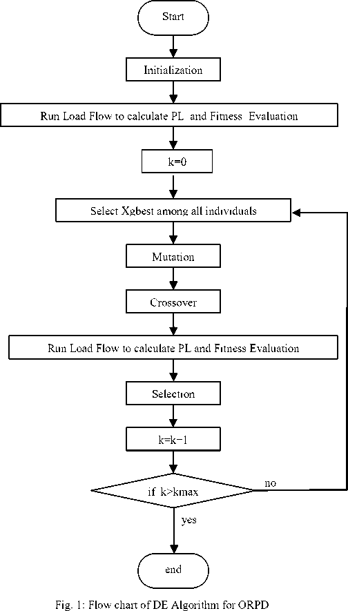
The procedure of the differential evolution optimization technique can be summarized in the flowchart of Fig. 1.

IV. Implementation of DE for Reactive PowerOptimal Dispatch

The details of the proposed algorithm are as follows:

• 4.3    Treatment of discrete variables

The discrete control variables are adjusting by 0.01 step size. Then each transformer tap setting is rounded to its nearest decimal integer value of 0.01, by utilizing the rounding operator. The same principle applies to the discrete reactive power injection of shunt compensators. The rounding operator is only performed in evaluating the fitness function.

The considered security constraints are the voltage magnitudes of all buses, the reactive power limits of the shunt VAR compensators and the transformers tap settings limits. The variables limits are listed in table 1.

Table 1: Initial Variables Limits (PU)

Control variables	Min. value	Max. value	Type
Generator: V g	0.90	1.10	continuous
Load Bus: V L	0.95	1.05	continuous
T	0.95	1.05	discrete
Q c	-0.12	0.36	discrete

The transformer taps and the reactive power source installation are discrete with the changes step of 0.01.

The power limits generators buses are represented in Table2. Generators buses are: PV buses 2,5,8,11,13 and slack bus is 1.the others are PQ-buses.

Table 2: Generators Power Limits in MW and MVAR

Bus n°	Pg	Pg min	Pg max	Qg min	Qg max
1	99.22	50	200	-20	200
2	80.00	20	80	-20	100
5	50.00	15	50	-15	80
8	20.00	10	35	-15	60
11	20.00	10	30	-10	50
13	20.00	12	40	-15	60

The total power demand is 283.4 Mw.

The DE population size is taken equal to 30. The maximum number of generations is 500, Mutation factor is F=0.7, and crossover rate is Rc=0.5, the penalty factors in equation (16) are chosen λ = 1000, λ = 500 . The weighting factor of voltage deviation is ω _v = 100 .

The complete algorithm has been implemented in Delphi oriented object programming. 20 runs have been performed for two cases of objective function and the results which follow are the best solution of these 20 runs.

• V. Simulation Results

DE algorithm has been tested on the IEEE 30-bus, 41 branch system [2,16]. It has a total of 13 control variables as follows: 6 generator-bus voltage magnitudes, 4 transformer-tap settings, and 2 bus shunt reactive compensators. Bus 1 is the slack bus, 2, 5, 8 , 11 and 13 are taken as PV generator buses and the rest are PQ load buses.

• Case1:    Active power loss minimization

  In this case1 only the minimization of active power loss is considered. The optimal settings of the control variables are given in table 3 case1 of DE. The total active power loss was initially 5.822 Mw and, it has been reduced by the proposed DE to 4.8752 Mw.

This solution is improved than the optimal active power loss obtained by the other heuristic methods reported in the literature with both continuous and discrete control variables such as standard genetic algorithm SGA[9] with 4.98 Mw, PSO[10] with 4.9262 Mw (table 4).

The total voltage deviation of PQ buses is VD=0.9619pu. The characteristic of convergence of DE algorithm is shown in fig. 2.

System of voltage profile of case1 and case 2 for all buses is shown in Fig.3. All voltage magnitudes of buses are within their limits, in PQ buses (load buses) voltage magnitude does not exceed its limits (1.05 and 0.95) except voltage magnitude at bus N°3, N°4, N°12 and N°27 of case 1 are 1.0563pu , 1.05079pu, 1.05205pu and 1.05041pu respectively.

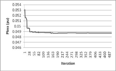
Fig. 2: Convergence characteristics

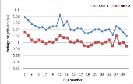
Fig. 3: Voltage profile diagram

• Case2:    Active power loss with voltage deviation minimization

  In the case 2, the minimization of voltage deviation is considered, the optimal settings of the control variables are given in table 3 case2 of DE. The total active power loss has been reduced by the proposed DE to 5.3700 Mw. The total voltage deviation of PQ buses is VD=0.18933 p.u.

Table 3: Values of Control Variables After Optimization and Active Power Loss

Control Variables (p.u)	Initial	DE Case1	DE Case2
V1	1.05	1.0774	1.0316
V2	1.04	1.0681	1.0211
V5	1.01	1.0457	1.0074
V8	1.01	1.0459	1.0017
V11	1.05	1.0851	1.0215
V13	1.05	1.0655	1.0133
T4,12	1.032	0.99	0.95
T6,9	1.078	1.03	1.04
T6,10	1.069	0.95	0.98
T28,27	1.068	0.97	0.95
Q10	0.00	0.14	0.27
Q24	0.00	0.11	0.12
PLOSS	5.822	4.8752	5.3988
VD	/	0.9619	0.1368

This result of VD is improved than the total voltage deviation VD of case 1.

It is clear that all control variables are within their boundary limits.

All voltage magnitudes of PQ buses are reduced in case 2 and approach to 1p.u.

The proposed approach succeeds in keeping the dependent variables within their limits.

Table 4 summarizes the results of the optimal solution obtained by PSO, SGA and DE methods. These results show that the optimal dispatch solution determined by the DE lead to lower active power loss than that found by GA method; witch confirms that DE is well capable of determining the global or near global optimum dispatch solution.

Table 4: Comparison Results of Different Methods

SGA[9]	PSO[10]	DE
4.98 Mw	4.9262Mw	4.8752Mw

• VI. Conclusion

In this paper, an efficient DE solution to the ORPF problem has been presented for determination of the global or near-global optimum solution for optimal reactive power dispatch with and without voltage deviation in PQ buses. The main advantages of the DE to the ORPD problem are optimization of different type of objective function, real coded of both continuous and discrete control variables, and easily handling nonlinear constraints. The proposed algorithm has been tested on the IEEE 30-bus system to minimize the active power loss. The optimal setting of control variables are obtained in both continuous and discrete value.

The results were compared with the other heuristic methods such as SGA and PSO algorithm reported in the literature and demonstrated its effectiveness and robustness.