Optimized and Self-Organized Fuzzy Logic Controller for pH Neutralization Process

Published Online November 2013 in MECS

pH control plays an important role in many industrial process applications such as wastewater treatment in paper and pulp plants, boiler feedwater treatment in thermal power plants, biopharmaceutical plants, food processing plants, and various other chemical processing plants. However, highly nonlinear titration curve with extreme sensitivity near to and extreme insensitivity away from the neutral pH of 7, and time varying parameters makes control of pH a very challenging problem. For these reasons, pH control is often regarded as a benchmark for modeling and control of highly nonlinear processes. In recent years the industrial application of advanced pH control techniques for the process industries has become more demanding, mainly due to the increasing complexity of the processes as well as due to stringent requirements of product quality and conformance with strict environmental and safety regulations. Therefore the process industries require more reliable, accurate, robust, and efficient pH control systems for the operation of process plants. In order to fulfill the above requirements there is a continuing need for research to develop advanced pH control schemes, many of which depend on accurate process model. The new trend in terms of advanced control technology is increasingly towards the use of a control approach known as an “intelligent” control strategy. Intelligent control can be described as a control approach or solution that tries to imitate important characteristics of the human brain and way of thinking and decision making. It is also a term that is commonly used to describe control schemes that are based on AI techniques such as neural networks, fuzzy logic, GAs, and their combinations.

The problem of pH control of neutralization process can be divided into two parts. The first part of the problem being the dynamic modeling of the pH neutralization process, whereas the second part being the design of appropriate control schemes based on the process model. Early works on pH control were based on development of the dynamic behavior of the pH process using the neutralization curve and its subsequent use in feedback, feedforward and ratio based adaptive control techniques [1]. The neutralization curves however are static in nature and subjected to variations if acid-base concentrations vary or buffering occurs. To overcome this difficulty the pH process is dynamically characterized as a first-order process with varying gain with or without dead time [2], [3]. Although time varying gain gave a better modeling alternative than static model, this model too was difficult to adopt, particularly in case of random variations in various process inputs. A more fundamental and rigorous approach for the development of the dynamic process model involves material balance on selective ions, equilibrium constants and electroneutrality equation [4], [5]. The associated model has been used by many researchers as a platform for subsequent investigations and forms the basis to introduce new and improved forms of dynamic modeling and adaptive control techniques using the concept of reaction invariant and strong acid equivalent [6], [7], [8], [9]. In addition to the first-principle based dynamic models, the other approaches have used the development of black-box type data-driven dynamic model based on AI techniques [10], [11], [12]. The main purpose in using AI techniques is to handle the inherent nonlinearity and time-varying nature of the pH neutralization process without the complex mathematical model, thereby improving its performance.

The advent of fuzzy set theory brought a phenomenal change in analysis of complex systems, decision processes and computational intelligence [13], [14]. The most visible paradigm shift was use of natural linguistic variables in place of numerical variables which resulted in “from computing with numbers to computing with words” [15]. The ascent was however not without resistance. During its nascent stage the term "fuzzy logic" gave an impression of vague logic and faced tremendous criticism from few leading scientific intellectuals. In reality, the term "fuzzy logic" refers to the fact that that the logic involved can deal with lexical definition of inputs, in contrast to binary logic which accepts only "true" or "false". Therefore, the term "fuzzy" in fuzzy logic applies to the imprecision in the data and not in the logic [16]. The fuzzy set theory laid the foundation of fuzzy control. The major boost to industrial application of fuzzy logic came with implementation of Mamdani fuzzy inference system based intelligent controller which provided a coherent strategy to combine linguistic control rules based on fuzzy theory [17]. Further to make the intelligent controller adaptive in nature, the self-organizing control strategies are applied [18], [19]. The extensive application of fuzzy logic to conventional control techniques such as proportional-integral-derivative control, sliding mode control, and adaptive control, resulted in improved performance for the hybrid controller over their conventional counterparts [20], [21], [22]. Apart from control applications, fuzzy logic has also been extensively used in system modeling identification [23], [24].

To optimize fuzzy inference system, various techniques are used. One among them is self-organizing technique in which the basic idea is to replace the poor performing rule with a better performing rule. Other techniques include altering fuzzy input-output scaling factors and membership functions with the help of evolutionary algorithms such as GA, a search techniques based on the mechanism of natural selection and natural genetics [25]. GAs perform evolutionary search within a defined search space as per “survival of fittest” principle proposed by Charles Darwin [26]. Over a number of years GAs have been extensively used in various optimization problems that are not well suited for standard optimization algorithms [27], [28], [29].

This research article is organized as follows. Section II describes the dynamic modeling of pH neutralization process. Section III introduces the design perspective of FLC. Section IV shows implementation of SOFLC. Section V gives methodology for genetic optimization of fuzzy inference system (FIS). Section VI details result and discussion on performance of FLC and SOFLC. Section VII presents the conclusion.

• II.    Dynamic Modeling of pH Neutralization Process

The pH neutralization process takes place in continuous stirred tank reactor (CSTR) with perfect mixing and constant volume. The CSTR has two influent streams: the hydrochloric acid as titration stream (feed A) and the sodium hydroxide as process stream (feed B), and one effluent stream. The flow characteristics of pump A and pump B are assumed to be linear and identical.

Stirrer

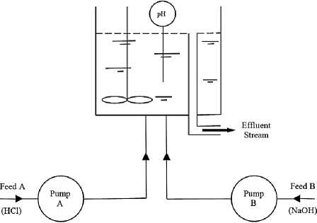
Fig. 1: pH neutralization process

The dynamic model of pH neutralization process involves material balances on selective ions, equilibrium relationship, and electroneutrality equation. Based on principle of material balances, the process mixing dynamics may be described as follows:

• V^= FaCa - (F a+Fb )x a (1)

• V Sr = FbCb - (F a+Fb )x b (2)

where V is the maximum volume of the CSTR (1.9 L); Ca is the concentration (0.05 mol/L) and Fa is the flow rate (0 to 6.23 mL/s i.e. 0 to 100%) of titration stream A;

C5 is the concentration (0.05 mol/L) and F5 is the flow rate (0 to 6.23 mL/s i.e. 0 to 100%) of process stream B; (Fа+F5 ) is the flow rate of the effluent stream; xа is the concentration of acid component (chloride ion, Cl ) in the effluent stream (in mol/L); xь is the concentration of base component (sodium ion, Na+ ) in the effluent stream (in mol/L).

The equilibrium relationship for water is given as

K = [H +][OH ](3)

where K is the dissociation constant of water (10-14).

From the electroneutrality condition, we have

[Na+]+ [H+]= [Cl ]+ [OH ](4)

All of the Cl ion comes from the HCl and all of the Na+ ion comes from the NaOH. Using (3) and (4), we have

[H +]2 - (x а- xb)[H+]- K =0(5)

From the definition of pH= -log10 [H +], the pH titration curve for a strong acid-strong base is given by pH= -log10 (1+ √+K )(6)

where x= (xа- xь )(7)

The block diagram implementation of dynamic pH neutralization process model is shown in Fig. 2.

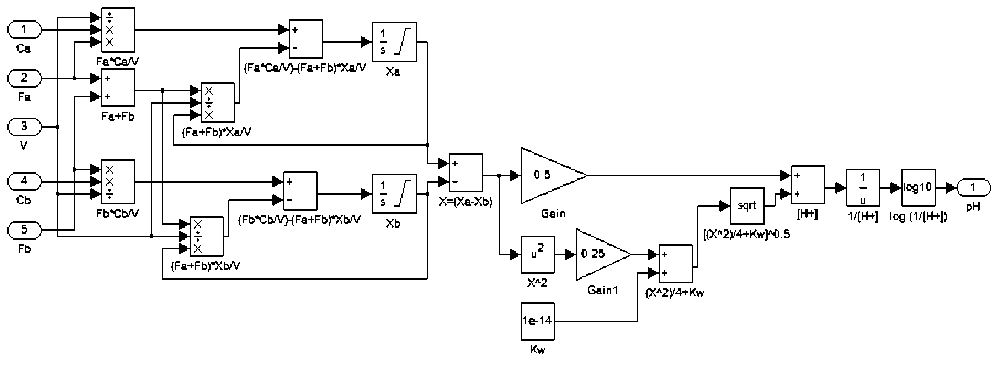
Fig. 2: Dynamic pH neutralization process model for strong acid-strong base

previous instant (k-1). The output variable for Sugeno FIS is co(k). Also another output variable co1(k) = Fа(k-1)-Fа (k) is used as minus of the change in manipulated variable i.e. minus of the change in acid flow rate of feed A. The relation between co(k) and co1(k) is shown in Fig. 6. The input variables are expressed in pH and output variables are expressed in %.

The linguistic variables for Sugeno FIS inputs (x^ =e and x2 =ce ) and output (y=co) are negative large (NL), negative medium (NM), negative small (NS), zero (ZE), positive small (PS), positive medium (PM), and positive large (PL). The definitions of the membership functions for input fuzzy sets are given in (8), (9), (10), (11), (12) and (13) where i = 1, 2, and m, n = 1, 2, 3, 4, 5, 6, 7 represents NL, NM, NS, ZE, PS, PM, PL respectively. Similarly the definition of the membership functions for output fuzzy set are given in (14) and (15) where q = 1, 2, 3, 4, 5, 6, 7 represents NL, NM, NS, ZE, PS, PM, PL respectively. The scaling factors k ,k2,k3 are real numbers. The universe of discourse for input fuzzy set is Х1 ∈ [-6,6] and output fuzzy set is У ∈ [0,1]. For k1 = k2 = k3 = 1, the shape of the membership functions for normalized inputs (e*, ce*) and output (co*) are shown in Fig. 3 and Fig. 4

respectively.

For xj ≤ -(4 - m)kj⁄3 and m = 1, we have

µim (x i)=1(8)

For -(5 - m)ki⁄3 ≤xi ≤ -(4 - m)ki⁄3 and m = 2, 3, 4, 5, 6, 7, we have

µim (x i)=^ [3xi+(5-m)ki ](9)

For xi ≥ -(3 - m)ki⁄3 and m = 1, 2, 3, 4, 5, 6, we have

µim (x i)=0(10)

For xj ≤ -(5 - m)kj⁄3 and m = 2, 3, 4, 5, 6, 7, we have

µim (x i)=0(11)

For -(4 - m)ki⁄3 ≤xi ≤ -(3 - m)ki⁄3 and m = 1, 2, 3, 4, 5, 6, we have

µim (x i)=-  [3xi+(3-m)ki](12)

For xi ≥ -(4 - m)ki⁄3 and m = 7, we have

µim (x i)=1(13)

For y= (ԛ- 1)k3⁄6 and q = 1, 2, 3, 4, 5, 6, 7, we have

µq(y) = 1(14)

For y≠ (ԛ- 1)k3⁄6 and q = 1, 2, 3, 4, 5, 6, 7, we have

µq(y) = 0(15)

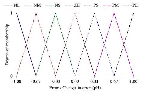
Fig. 3: Normalized membership functions for error and change in error

---N 1 1 E h Q 0 0.	IL .........^	IM -----	MS---	;e -■-	>S--F	M---PL 1 i i i i i i i ______________________________i
	DO      0.17      0.33      0.50      0.67      0.					83      1.00

Change in output (%)

Fig. 4: Normalized membership functions for change in output

Table 1:  Fuzzy Rule Base

e	ce
	NL	NM	NS	ZE	PS	PM	PL
NL	MF 11	MF 12	MF 13	MF 14	MF 15	MF 16	MF 17
NM	MF 21	MF 22	MF 23	MF 24	MF 25	MF 26	MF 27
NS	MF 31	MF 32	MF 33	MF 34	MF 35	MF 36	MF 37
ZE	MF 41	MF 42	MF 43	MF 44	MF 45	MF 46	MF 47
PS	MF 51	MF 52	MF 53	MF 54	MF 55	MF 56	MF 57
PM	MF 61	MF 62	MF 63	MF 64	MF 65	MF 66	MF 67
PL	MF 71	MF 72	MF 73	MF 74	MF 75	MF 76	MF 77

MF 11 , MF 12 , MF 13 , MF 14 , MF 21 , MF 22 , MF 23 , MF 31 , MF 32 , MF 41 ≡ NL; MF 15 , MF 24 , MF 33 , MF 42 , MF 51 ≡ NM; MF 16 , MF 25 , MF 34 , MF 43 , MF 52 , MF 61 ≡ NS; MF 17 , MF 26 , MF 35 , MF 44 , MF 53 , MF 62 , MF 71 ≡ ZE; MF 27 , MF 36 , MF 45 , MF 54 , MF 63 , MF 72 ≡ PS; MF 37 , MF 46 , MF 55 , MF 64 , MF 73 ≡ PM; MF 47 , MF 56 , MF 57 , MF 65 , MF 66 , MF 67 , MF 74 , MF 75 , MF 76 , MF 77 ≡ PL.

To frame fuzzy rule (FR) base, let us suppose x 1 = NL and x 2 = NL. Here x 1 = NL implies that pH(k) >> pH_SP i.e. the present pH is much away from the setpoint and x₂ = NL implies that pH(k) >> pH(k-1) i.e. the pH response has tendency to move away from the setpoint. Therefore to bring pH back to the setpoint we must increase the acid flow rate by large amount. Similarly, let us suppose next x 1 = NL and x 2 = PL. Here x 1 = NL implies that pH(k) >> pH SP i.e. the present pH is much away from the setpoint and x 2 = PL implies that pH(k) << pH(k-1) i.e. the pH response has tendency to move towards the setpoint. Therefore to bring pH back to the setpoint we must keep the acid flow rate unchanged. The complete fuzzy rule base for FLC is shown in Table I. The individual fuzzy rule structure is represented by

FRz: IF x1 is m AND x2 is n THEN y is MFmn where z = (7m + n - 7), and m, n = 1, 2, 3, 4, 5, 6, 7 represents NL, NM, NS, ZE, PS, PM, PL respectively.

The defuzzified output of the FLC (yFC) is given by (16).

y_F c (xi,x ₂ )

²n - 1 2 m - i^{[{ m} i ⁿ⁽ H 1 m^(x 1 ), H 2 n ^(x 2 ))} ^{M F} mn ] 2n -1 2 m -1 { ^m iⁿ( H 1 m ⁽X 1 ) H 2 nfe ))}

• IV.    Design of SOFLC

The FLC for inherently nonlinear pH neutralization process can be optimized for a given operating condition. However the controller needs to be reoptimized if the operating condition changes. This necessitates development of adaptive controller which have adjustable parameters and a mechanism for adjusting the parameters [31]. To make the FLC performance adaptive, the self-organizing technique is incorporated using performance correction table (PC) shown in Table II where k is a positive scaling factor. The self-organizing strategy uses non-zero penalties for non-performance and zero penalties for meeting performance. We know if -6 <  x 1 <  -2.5 and -6 <  x ₂ <  -2.5, then the pH response is moving away from the setpoint and to bring pH back to the setpoint we must increase the acid flow rate. Therefore we can impose a non-zero penalty on each output membership functions which will result in more increase in acid flow rate. Similarly if -6 <  x 1 <  -2.5 and 0.5 <  x₂ <  6, then we will impose zero penalties on each output membership functions since the pH response is already moving towards the setpoint.

The self-organizing mechanism updates FLC output membership as per following rule.

If -6 <  x 1 <  -2.5 and -6 <  x₂ <  -2.5, then

MF mn (new) = MF mn (old) + PC_n x 10 - ⁵

If -6 <  x 1 <  -2.5 and -2.5 <  x₂ <  -1.5, then

MF mn (new) = MF mn (old) + PC₁₂ x 10 - ⁵

If -6 <  x 1 <  -2.5 and -1.5 <  x₂ <  -0.5, then

MF mn (new) = MF mn (old) + PC₁₃ x 10 - ⁵

If -6 <  x 1 <  -2.5 and -0.5 <  x₂ <  0.5, then

MF mn (new) = MF mn (old) + PC₁₄ x 10 - ⁵

If -2.5 <  x 1 <  -1.5 and -6 <  x₂ <  -2.5, then

MF mn (new) = MF mn (old) + PC₂₁ x 10 - ⁵

If -2.5 <  x 1 < -1.5 and -2.5 <  x₂ <  -1.5, then

MF mn (new) = MF mn (old) + PC₂₂ x 10 - ⁵

If -2.5 <  x 1 <  -1.5 and -1.5 <  x 2 <  -0.5, then

MF mn (new) = MF mn (old) + PC₂₃ x 10 - ⁵

If -2.5 <  x 1 <  -1.5 and -0.5 <  x 2 <  0.5, then

MF mn (new) = MF mn (old) + PC 24 x 10^-5

If -1.5 <  x 1 <  -0.5 and -6 <  x 2 <  -2.5, then

MF mn (new) = MF mn (old) + PC 31 x 10^-5

If -1.5 <  x 1 <  -0.5 and -2.5 <  x 2 <  -1.5, then

MF mn (new) = MF mn (old) + PC₃₂ x 10 - ⁵

If -1.5 <  x 1 <  -0.5 and -1.5 <  x₂ <  -0.5, then

MF mn (new) = MF mn (old) + PC₃₃ x 10 - ⁵

If -1.5 <  x 1 <  -0.5 and -0.5 <  x₂ <  0.5, then

MF mn (new) = MF mn (old) + PC 34 x 10 - ⁵

If -0.5 <  x₁ <  0.5 and -6 <  x₂ <  -2.5, then

MF_mn(new) = MF_mn(old) + PC₄₁ x 10^-5

If -0.5 <  x₁ <  0.5 and -2.5 <  x₂ <  -1.5, then

MF_mn(new) = MF_mn(old) + PC₄₂ x 10^-5

If -0.5 <  x₁ <  0.5 and -1.5 <  x₂ <  -0.5, then

MF mn (new) = MF mn (old) + PC 43 x 10 - ⁵

If -0.5 <  x 1 <  0.5 and 0.5 <  x₂ <  1.5, then

MF mn (new) = MF mn (old) + PC₄₅ x 10^-5

If -0.5 <  x 1 <  0.5 and 1.5 <  x₂ <  2.5, then

MF mn (new) = MF mn (old) + PC 46 x 10 - ⁵

If -0.5 <  x 1 <  0.5 and 2.5 <  x 2 <  6, then

MF mn (new) = MF mn (old) + PC 47 x 10^-5

If 0.5 <  x 1 <  1.5 and -0.5 <  x₂ <  0.5, then

MF mn (new) = MF mn (old) + PC₅₄ x 10^-5

If 0.5 <  x 1 <  1.5 and 0.5 <  x₂ <  1.5, then

MF mn (new) = MF mn (old) + PC₅₅ x 10^-5

If 0.5 <  x 1 <  1.5 and 1.5 <  x₂ <  2.5, then

MF mn (new) = MF mn (old) + PC 56 x 10 - ⁵

If 0.5 <  x 1 <  1.5 and 2.5 <  x₂ <  6, then

MF mn (new) = MF mn (old) + PC 57 x 10^-5

If 1.5 <  x 1 <  2.5 and -0.5 <  x₂ <  0.5, then

MF mn (new) = MF mn (old) + PC 64 x 10^-5

If 1.5 <  x 1 <  2.5 and 0.5 <  x₂ <  1.5, then

MF mn (new) = MF mn (old) + PC 65 x 10 - ⁵

If 1.5 <  x 1 <  2.5 and 1.5 <  x₂ <  2.5, then

MF mn (new) = MF mn (old) + PC 66 x 10 - ⁵

If 1.5 <  x₁ <  2.5 and 2.5 <  x₂ <  6, then

MF mn (new) = MF mn (old) + PC 67 x 10 - ⁵

If 2.5 <  x 1 <  6 and -0.5 <  x 2 <  0.5, then

MF mn (new) = MF mn (old) + PC₇₄ x 10^-5

If 2.5 <  x 1 <  6 and 0.5 <  x₂ <  1.5, then

MF mn (new) = MF mn (old) + PC₇₅ x 10^-5

If 2.5 <  x 1 <  6 and 1.5 <  x ₂ <  2.5, then

MF mn (new) = MF mn (old) + PC 76 X 10^-5

If 2.5 <  x 1 <  6 and 2.5 <  x₂ <  6, then

MF mn (new) = MF_mn(old) + PC₇₇ x 10^-5

where m, n = 1, 2, 3, 4, 5, 6, 7, and PC mn are the elements of fuzzy performance correction table as shown in Table II.

Table 2:  Performance Correction Table

e	ce
	-6 to -2.5	-2.5 to -1.5	-1.5 to -0.5	-0.5 to 0.5	0.5 to 1.5	1.5 to 2.5	2.5 to 6
-6 to -2.5	-3k	-3k	-3k	-3k	0	0	0
-2.5 to -1.5	-3k	-2k	-2k	-2k	0	0	0
-1.5 to -0.5	-2k	-2k	-1k	-1k	0	0	0
-0.5 to 0.5	-2k	-1k	-1k	0	1k	1k	2k
0.5 to 1.5	0	0	0	1k	1k	2k	2k
1.5 to 2.5	0	0	0	2k	2k	2k	3k
2.5 to 6	0	0	0	3k	3k	3k	3k

• V.    FIS Optimization using GA

The flowchart for GA optimization of FIS, conventional or self-organized, is shown in Fig. 5 [32]. To optimize the FIS, the scaling factors k 1 , k 2 , and k 3 are chosen to proportionately scale the vertices of membership functions for normalized variables e*, ce*, and co* respectively as given in (8), (9), (10), (11), (12), (13), (14) and (15). To optimize the performance correction table, the scaling factor k is chosen.

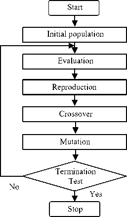
Fig. 5: Flowchart for GA optimization

GA optimization starts with an initial population of individuals of type ‘double’ and size ‘20’, generated at random within the initial population range representing minimum and maximum values for optimization variables. Each individual in the population represents a potential solution to the optimization problem under consideration. The individuals evolve through successive iterations, called generations. During each generation, each individual in the population is evaluated using integral of squared errors (ISE) fitness function. The evaluated fitness values of the individuals are ranked in an increasing order such that the best elite individual having minimum fitness value has the rank as1, the next elite individual fit has the rank as 2, and so on. The rank fitness scaling function is used to assign scaled values to the individuals inversely proportional to square root of their rank. Based on the assigned scaled values by the fitness scaling function, the selection function is used to select parents for next generation. The stochastic uniform selection function represents a line in which each parent corresponds to a section of the line of length proportional to its scaled value. The GA moves along the line in steps of equal size and, at each step, the GA allocates a parent to the section it occupies. Using current generation individuals, the next generation population is created through genetic operators namely reproduction, crossover and mutation. The reproduction operation has the elite children count as 2. Besides elite children, the GA uses current generation parents to create next generation crossover and mutation children. The GA creates the crossover children by combining a pair of parents whereas the mutation children are created by applying random changes to a single parent. The GA uses scattered crossover with fraction as 0.8 to create 14 crossover children. The remaining 4 next generation children are created using Gaussian mutation with both scale and shrink as 0.01. The procedure continues until the termination condition is satisfied. The GA optimization parameters are given in Table III. Unless otherwise indicated, the values are true for servo and regulatory operations of both FLC and SOFLC.

• VI.    Simulation Results and Discussions

• 6.1 Servo Response

The schematic block diagram for implementation and optimization of SOFLC for pH neutralization process is shown in Fig. 6. The output membership functions for variable ‘co’ are placed within the range [0,k ] for conventional FLC, as given in (14) and (15). The output membership functions for variable ‘co1’ are placed within the range [-40k ,40k ] . The performance of optimized "intelligent" controller, conventional as well as self-organized, are compared for servo and regulatory operations based on ISE, maximum overshoot and undershoot, settling and rejection time (for ± 2% pH error band) using MATLAB simulation. To calculate ISE, all the errors with magnitude greater than or equal to 0.01 are considered since further smaller errors will have negligible contribution.

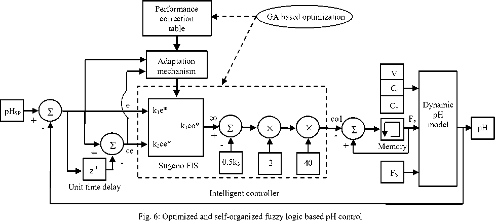
Table 3:  GA Optimization Parameters

Parameters	Descriptions
Variables	(k 1 , k 2 , k 3 ) FLC (k 1 , k 2 , k 3 , k) SOFLC
Population	Type: Double vector Size: 20 Creation function: Uniform Initial range: [0 0 0;4.5 4.5 0.03] FLC Servo [0 0 0;4.5 4.5 0.05] FLC Regulatory [0 0 0 0;4.5 1.5 0.02 0.05] SOFLC Servo [0 0 0 0;4.5 4.5 0.06 0.08] SOFLC Regulatory
Fitness scaling	Function: Rank
Selection	Function: Stochastic uniform
Reproduction	Elite count: 2 Crossover fraction: 0.8
Mutation	Function: Gaussian Scale: 0.01 Shrink: 0.01
Crossover	Function: Scattered
Migration	Direction: Forward Fraction: 0.2 Interval: 20
Constraint parameters	Initial penalty: 10 Penalty factor: 100
Stopping criteria	Generations: 100 Stall generations: 50 Function tolerance: 10-6

For servo operation, the pH setpoint (pHSP) variation is shown below for various sampling instants (k).

For 1≤k≤600, we have рН (k)=7

For 601≤k≤1200, we have рН (k)=8

For 1201≤k≤1800, we have рН (k)=9

For 1801≤k≤2400, we have рН (k)=8

For 2401≤k≤3000, we have рН (k)=7

For 3001≤k≤3600, we have рН (k)=6

For 3601≤k≤4200, we have рН (k)=5

For 4201≤k≤4800, we have рН (k)=6

For 4801≤k≤5400, we have рН (k)=7

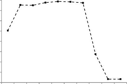
The process variable Fb is kept constant at 1.75 mL/s. The self-organization adaptation loop is set to run for 10 iterations. The plot of best and mean values of ISE as a result of GA optimization process for FLC and SOFLC are shown in Fig. 7 and Fig. 8. The final mean fitness values are closer to best fitness values which indicate good GA convergence. The resulting values of scaling factors k1, k2. k3, and k are given in Table IV. The performance characteristic of self-organization technique is shown in Fig. 9. The variations of controlled and manipulated variables for servo response for selected duration are shown in Fig. 10 and 11 respectively.

Best fitness value                                               ^{Best fitness value}

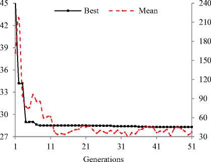
Fig. 7: GA optimization for FLC (servo response)

Fig. 8: GA optimization for SOFLC (servo response)

1     2     3     4     5     6     7     8     9    10

Iteration number

Fig. 9: Self-organizing performance characteristic for servo response

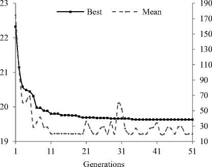
Table 4:  Comparison of Servo Response

Parameters	FLC	SOFLC
k1	4.74203	3.56715
k2	0.85630	0.49444
k3	0.01113	0.01576
k	0	0.04646
ISE	28.2985	19.6285
Maximum undershoot*1	0.87818	0.27198
Maximum overshoot*2	0.87896	0.27122
Settling time*1	28 samples	15 samples
Settling time*2	28 samples	15 samples

*¹ For pH SP changes from 9 to 8. *² For pH SP changes from 5 to 6.

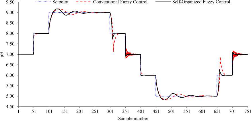
Fig. 10: Controlled variable variations for servo response for selected duration

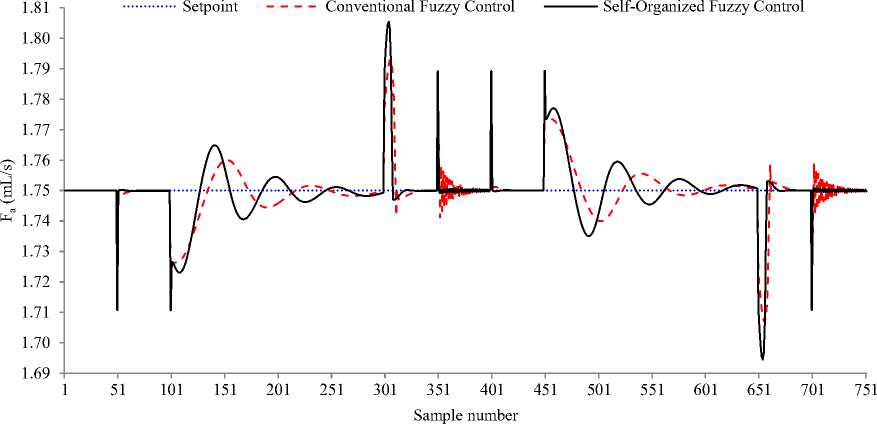
Fig. 11: Manipulated variable variations for servo response for selected duration

In comparison with FLC, the SOFLC demonstrates superior servo performance as indicated by values in Table IV. The self-organization mechanism reduces the ISE by almost 30%. Both controllers shows worst performance when the pH SP changes from 9 to 8 and from 5 to 6. However SOFLC again outperforms FLC by reducing maximum undershoot and overshoot by 69%. Finally the SOFLC reduces the settling time by 46% in comparison with FLC.

The self-organization mechanism essentially modifies the output membership functions M 33 , M 34 , M 43 , M 44 , M 45 , M 54 , and M 55 as indicated in Table VI.

• 6.2    Regulatory Response

For regulatory operation, the process variable F b (in mL/s) variation is shown below for various sampling instants (k).

For 1≤k≤600, we have F5(k) = 1.75

For 601≤k≤1200, we have Fb(k) = 1.8375

For 1201≤k≤1800, we have Fb (k) = 1.75

For 1801≤k≤2400, we have Fb (k) = 1.6625

For 2401≤k≤3000, we have F5 (k) = 1.75

For 3001≤k≤3600, we have F5 (k) = 1.925

For 3601≤k≤4200, we have F5 (k) = 1.75

For 4201≤k≤4800, we have Fb (k) = 1.575

For 4801≤k≤5400, we have Fb (k) = 1.75

The setpoint pHSP is kept constant at 7. The selforganization adaptation loop is set to run for 10 iterations. The plot of best and mean values of ISE as a result of GA optimization process for FLC and SOFLC are shown in Fig. 12 and Fig. 13. The final mean fitness values are closer to best fitness values which again indicate good GA convergence for the regulation. The resulting values of scaling factors k1, k2. k3, and k are given in Table IV. The performance characteristic of self-organization technique is shown in Fig. 14. The variations of controlled and manipulated variables for regulatory response for selected duration are shown in Fig. 15 and 16 respectively.

In comparison with FLC, the SOFLC demonstrates superior regulatory performance as indicated by values in Table IV. The self-organization mechanism reduces the ISE by almost 30%. Both controllers show almost equal maximum undershoot and overshoot when process is subjected to disturbance of ± 10%. Finally the SOFLC reduces the settling time by more than 60% in comparison with FLC.

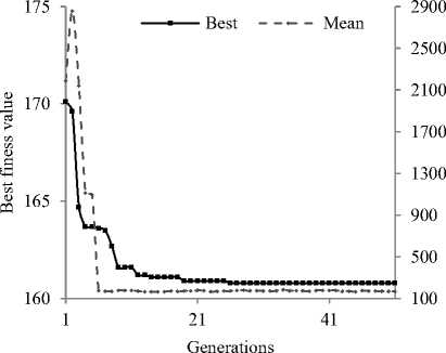
Fig. 12: GA optimization for FLC (regulatory response)

Best finess value

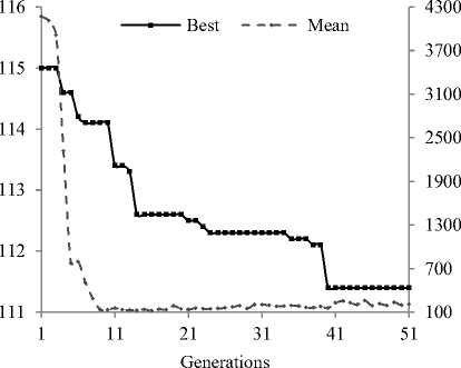
Fig. 13: GA optimization for SOFLC (regulatory response)

1800      \ й 1200           \

\

1     2     3     4    5     6    7     8     9    10

Iteration number

Fig. 14: Self-organizing performance characteristics for regulatory response

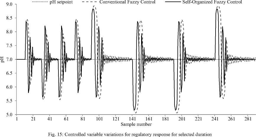
Table 5:  Comparison of Regulatory Response

Parameters	FLC	SOFLC
k1	4.45597	1.95117
k2	3.95831	3.19950
k3	0.03984	0.03792
k	0	0.07132
ISE	160.782	111.377
Maximum undershoot*1	1.94240	1.82714
Maximum overshoot*2	1.94209	1.82710
Rejection time*1	111 samples	44 samples
Rejection time*2	114 samples	33 samples

*¹ For F B changes by -10%. *² For F B changes by +10%.

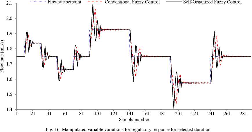
Table 6: Modification of Fuzzy Rule Base

e	ce
	NL	NM	NS	ZE	PS	PM	PL
NL	0	0	0	0	0.00189	0.00379	0.00557	FLC Servo
	0	0	0	0	0.00677	0.01355	0.01992	FLC Regulatory
	0	0	0	0	0.00268	0.00536	0.00788	SOFLC Servo*1
	0	0	0	0	0.00268	0.00536	0.00788	SOFLC Servo*2
	0	0	0	0	0.00645	0.01289	0.01896	SOFLC Regulatory*1
	0	0	0	0	0.00645	0.01289	0.01896	SOFLC Regulatory*2
NM	0	0	0	0.00189	0.00379	0.00557	0.00735	FLC Servo
	0	0	0	0.00677	0.01355	0.01992	0.02629	FLC Regulatory
	0	0	0	0.00268	0.00536	0.00788	0.01040	SOFLC Servo*1
	0	0	0	0.00268	0.00536	0.00788	0.01040	SOFLC Servo*2
	0	0	0	0.00645	0.01289	0.01896	0.02503	SOFLC Regulatory*1
	0.00000	0.00000	0.00000	0.00637	0.01289	0.01896	0.02503	SOFLC Regulatory*2
NS	0	0	0.00189	0.00379	0.00557	0.00735	0.00924	FLC Servo
	0	0	0.00677	0.01355	0.01992	0.02629	0.03307	FLC Regulatory
	0	0	0.00268	0.00536	0.00788	0.01040	0.01308	SOFLC Servo*1
	0	0	0.00402	0.00534	0.00788	0.01040	0.01308	SOFLC Servo*2
	0	0	0.00645	0.01289	0.01896	0.02503	0.03147	SOFLC Regulatory*1
	0.00000	0.00000	0.00916	0.01297	0.01900	0.02503	0.03147	SOFLC Regulatory*2
ZE	0	0.00189	0.00379	0.00557	0.00735	0.00924	0.01113	FLC Servo
	0	0.00677	0.01355	0.01992	0.02629	0.03307	0.03984	FLC Regulatory
	0	0.00268	0.00536	0.00788	0.01040	0.01308	0.01576	SOFLC Servo*1
	0	0.00268	0.00690	0.00788	0.00885	0.01308	0.01576	SOFLC Servo*2
	0	0.00645	0.01289	0.01896	0.02503	0.03147	0.03792	SOFLC Regulatory*1
	0	0.00645	0.01653	0.01897	0.02142	0.03148	0.03792	SOFLC Regulatory*2
PS	0.00189	0.00379	0.00557	0.00735	0.00924	0.01113	0.01113	FLC Servo
	0.00677	0.01355	0.01992	0.02629	0.03307	0.03984	0.03984	FLC Regulatory
	0.00268	0.00536	0.00788	0.01040	0.01308	0.01576	0.01576	SOFLC Servo*1

PS	0.00268	0.00536	0.00788	0.01042	0.01176	0.01576	0.01576	SOFLC Servo*2
	0.00645	0.01289	0.01896	0.02503	0.03147	0.03792	0.03792	SOFLC Regulatory*1
	0.00645	0.01289	0.01891	0.02496	0.02872	0.03792	0.03792	SOFLC Regulatory*2
PM	0.00379	0.00557	0.00735	0.00924	0.01113	0.01113	0.01113	FLC Servo
	0.01355	0.01992	0.02629	0.03307	0.03984	0.03984	0.03984	FLC Regulatory
	0.00536	0.00788	0.01040	0.01308	0.01576	0.01576	0.01576	SOFLC Servo*1
	0.00536	0.00788	0.01040	0.01308	0.01576	0.01576	0.01576	SOFLC Servo*2
	0.01289	0.01896	0.02503	0.03147	0.03792	0.03792	0.03792	SOFLC Regulatory*1
	0.01289	0.01896	0.02503	0.03155	0.03792	0.03792	0.03792	SOFLC Regulatory*2
PL	0.00557	0.00735	0.00924	0.01113	0.01113	0.01113	0.01113	FLC Servo
	0.01992	0.02629	0.03307	0.03984	0.03984	0.03984	0.03984	FLC Regulatory
	0.00788	0.01040	0.01308	0.01576	0.01576	0.01576	0.01576	SOFLC Servo*1
	0.00788	0.01040	0.01308	0.01576	0.01576	0.01576	0.01576	SOFLC Servo*2
	0.01896	0.02503	0.03147	0.03792	0.03792	0.03792	0.03792	SOFLC Regulatory*1
	0.01896	0.02503	0.03147	0.03792	0.03792	0.03792	0.03792	SOFLC Regulatory*2

*1 - Before adaptation mechanism

*2 - After adaptation mechanism

The self-organization mechanism essentially modifies the output membership functions M₂₁, M₂₂, M 23 , M 24 , M 31 , M 32 , M 33 , M 34 , M 35 , M 42 , M 43 , M 44 , M 45 , M 46 , M 53 , M 54 , M 55 , M 56 , M 57 , M 64 , M 65 , M 66 , and M 67 as indicated in Table VI.

• VII. Conclusion

  In this paper, the intelligent controller for pH neutralization process is designed by incorporating the self-organizing mechanism in the conventional FLC to make it performance adaptive. The SOFLC adaptation mechanism modifies the output membership function positions using performance correction table. In order to have optimal performance, parameters of both FLC as well as SOFLC are optimized using GA. In case of servo response, the ISE and maximum undershoot and overshoot for SOFLC are decreased in comparison with FLC, by approximately 30% and 69% respectively. Also, the settling time for servo response is reduced by 46% for SOFLC in comparison with FLC. Similarly, in case of regulatory response, the ISE and the rejection time for SOFLC are less by approximately 30% and 5060% respectively, in comparison with FLC.