Orbit and Attitude Control of Asymmetric Satellites in Polar Near-Circular Orbit

Author: Wei Zhao, Weiwei Yang, Xiaoqian Chen, Yong Zhao
Journal: International Journal of Intelligent Systems and Applications(IJISA) @ijisa
Article in issue: 1 vol.1, 2009.
Free access
In this paper, the general problem about the orbit and attitude dynamic model is discussed. A feedback linearization control method is introduced for this model. Due to the asymmetric structure, the orbital properties of such satellites are the same as traditional symmetric ones, but the attitude properties are greatly different from the symmetric counterparts. With perturbations accumulate with time, the attitude angles increase periodically with time, but the orbital elements change much slower than the attitude angles. In the attitude dynamic model, chaos could appear. Traditional linear controllers can not compensate enough for asymmetric satellite when the mission is complex, especially in maneuver missions. Thus nonlinear control method is required to solve such problem in large scale. A feedback linearization method, one robust nonlinear control method, is introduced and applied to the asymmetric satellite in this paper. Some simulations are also given and the results show that feedback linearization controller not only stabilizes the system, but also exempt the chaos in the system.
Asymmetric satellite, orbit control, attitudecontrol, feedback linearization, chaos
Short address: https://sciup.org/15010074
IDR: 15010074
Text of the scientific article Orbit and Attitude Control of Asymmetric Satellites in Polar Near-Circular Orbit
Published Online October 2009 in MECS
With the development of aerospace technology, more and more advanced instruments are equipped in one satellite to accomplish complex missions. Some satellites are designed to have asymmetric configuration with only one solar array in order to avoid sheltering the payload.
As shown in Fig. 1, the second-generation of meteorological satellite FY-3 in China, is equipped with 10 channels of scanning radiometers, 20 channels of infrared spectrometers, 20 channels of medium-resolution imaging spectrometers, vertical ozone detector, total ozone detector, solar radiation measuring instrument, 4channels of microwave temperature detectors, 5 channels of microwave moisture meters, microwave imaging device, Earth radiation instrument, and space environment surveillance camera. It is impossible for the traditional symmetric satellite to have so many payloads equipped. However, the control strategy for such kind of satellites is also challenging. ETS-VII in Japan and Orbit
Manuscript received January 22, 2009; revised June 13, 2009; accepted July 21, 2009.
Express in the US are also designed as asymmetric structure for the same reason.
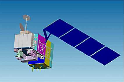
Figure 1. FY-3 meteorological satellite in China.
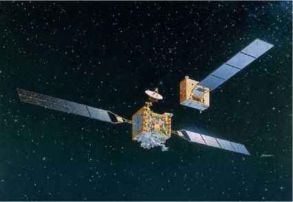
Figure 2. ETS-VII and its demonstration of rendezvous
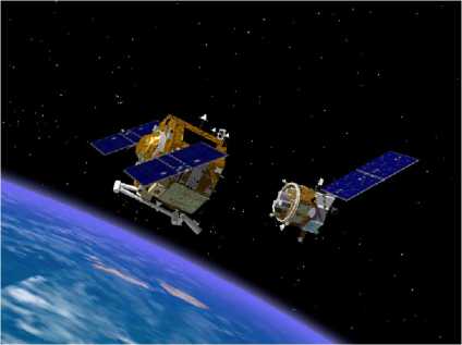
Figure 3. Orbit Express and its demonstration of rendezvous
For the satellites with symmetric structure, perturbation moments are approximately zero. The disturbance to attitude angle is very small and can be neglected in the attitude controller design procedure. But for the asymmetric satellites, perturbation moments may accumulate with time, and cannot be ignored especially in the long run. The asymmetric satellites may need a nonzero torque equilibrium attitude. The accumulation of perturbation moments can even cause chaos in attitude dynamic system. Traditional linear attitude controller may not compensate enough when the mission is complex, such as maneuver and rendezvous, because the working state of the satellite is far from design equilibrium point. Thus traditional linear controller can not perform well enough or even cause instability. Nonlinear control strategy should be introduced to solve this attitude control problem in such circumstances. Feedback linearization is a nonlinear control method, easy to be implemented, and its robustness has been proved in some recent researches [2]. In this paper, it will be adopted to design the orbit controller and the attitude controller.
The paper is organized in the following way: in Section 2, orbit dynamic model is introduced. Attitude dynamic model for asymmetric satellite is given in Section 3; Section 4 presents an analysis of the property of the attitude dynamics for this kind of satellite without control; A feedback linearization method is introduced in Section 5 and it is applied to the forward model to design the control law for the attitude determination and control system (ADCS), the simulation results are also shown as well; In Section 6 conclusions and suggestions of future work are given.
-
II. O RBIT D YNAMIC M ODEL
The orbital plane of a satellite in polar orbit is almost perpendicular along the direction from the sun to the earth. с denotes the angle between the norm of the orbital plane and the line from the sun to the earth. The eccentricity of the orbit is very small.
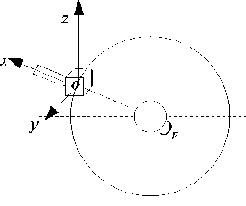
Figure 4. Orbit, nominal attitude and the axes of the asymmetric satellite
The disturbance forces caused by Earth Non-Sphericity, aerodynamics, solar radiate pressure are discussed in the following paragraphs. Because the disturbance force caused by the earth's magnetic force is zero, this factor is not discussed. Considering all the disturbance forces, the Orbit dynamic model of asymmetric satellite is as follows:
d v ^ m v v v v
-
— =- — v0 + R g + R a + R s + R c (2.1)
dt r 2
Where, v 0 denotes the unit vector of from center of the
Earth to mass center of the satellite; Rg denotes the
v disturbance force of Earth Non-Sphericity; Ra denotes the
v disturbance force of aerodynamics; RS denotes the
v disturbance force of solar radiate pressure; Rc denotes the control force.
Orbital elements are six key constants for the two-body problem. Using the orbital elements as basic variable, orbit disturbance equation can be written as follows [4]:
* = —[ e sin f g f + ( 1+ e cos f ) f J
na 2V1 - e2
f h
<
r sin u
2 2 fh na \1 - e sin i

nae
M = n
^^^^^^»
I P J
- cos i g Q
1 - e 2
nae
2 er - cos f I f r +11 + r | sin f g ft
(2.2)
Where, a denotes semi-major axis of the orbit; e denotes the eccentricity of the orbit; i denotes the orbit inclination angle; Q denotes the right ascension of the ascending node (RAAN); ® denotes the argument of perigee; M denotes the mean anomaly; f denotes the true anomaly; E denotes the eccentric anomaly; u = f + ® ; n denotes the average angular velocity; r denotes the distance between the mass center of satellite and the center of the earth; P = a (1 - e2 ) ;
fr denotes the disturbance force along the radial direction;
ft denotes the disturbance force along the lateral direction; fh denotes the disturbance force along the norm of orbit.
Some complementary equations for the Equ. (2.2) are also written as follows.
E - e sin E = M (Kepler Equation)
f 1+e E tan— = tan—
2 V1- e 1
a 3
V ^g
-
1 + e cos f
(2.3)
(2.4)
(2.5)
(2.6)
-
A. Disturbance Force of Earth Non-Sphericity
Earth flattening J 2 is the main item of the disturbance that affects the orbit of the satellite. The corresponding disturbance force is as follows [4]:
R g =- JE" ( 3sin 2 Ф — 1 ) V 0 (2.7)
Where, aE denotes the Earth equatorial radius;
J 2 = 1.082626 x10 - 3 denotes the coefficient of the disturbance item; ф denotes the geocentric latitude;
V 0 denotes the unit vector from the center of Earth to the satellite.
The relationship between the geocentric latitude and the orbital elements is as follows:
sin ф = sin i sin ( f + m )
(2.8)
v
Ra = - £V^CDAlpV (2.11) v
Where, Ra denotes the aerodynamic force, p 1 denotes the density of local atmosphere, VR denotes the satellite velocity, CD denotes the drag coefficient, Ap denotes the surface area, v v = - n v a denotes the unit vector of the satellite.
Local density of the atmosphere calculated by the exponential atmosphere model, which is written as follows:
The disturbance caused by the Earth Non-Sphericity includes long-time item, long-period item, and shortperiod item. Because J 2 item does not contain long-period item, R can be divided into a long-time item and a short-period item. The short-period item fluctuates very quickly with time, while long-time item will accumulate with time, so only the long-time item should be considered here.
For conservative forces, the disturbed orbital elements
can be written as follows[4]:
L 2 dR a =—
P 1 = P 10 e" H° (2.12)
Where, p 10 = 3.6 x10 - 10 kg g m - 3 ; H = 37.4 km ;
r 0 = H + 6371 km .
Velocity of the satellite in the orbit axis is as follows:
v V a 2 n V a 2 n
VR =--sin E g P +-- V1 - e cos E g Q (2.13)
rr cos Q cos m - sin Q sin mcos i v
Where, P = sin Q cos m + cos Q sin m cos i , sin m sin i
e=
na dM
1 - e 2 d R ^ 1 - e 2 d R
£= na
na 2 e d M
na 2 e dm
( JRR dR
- cos Q sin m - sin Q cos m cos i
V
Q = - sin Q sin m + cos Q cos m cos i cos m sin i
2 V1 - e 2 sin i vr- e 2
d R
(2.9)
m =---2-- na e de
M = n
1 - e 2 d R
. dQ cosi dt
Because the surface of the solar array is much larger than the satellite main body, the surface area of the main body can be ignored in the calculation.
The surface of the solar array can be written as:
A = ab |sin ^ ) + ab |cos ^ k (2.14)
The unit vector of incoming flow can be considered as the inverse direction of the velocity of satellite, so we have:
na 2 e de na da
For the disturbance caused only by the Earth NonSphericity, the disturbance equations can be simplified as follows:
V
V Vr v = —
V R
(2.15)
Then we get
A p = l A g vl
(2.16)
£= 0
3 J 2 aE 2 2 p 2 n 3
cos i
(2.10)
3 J 2 aE 2 2 p 2 n 3
(- 5-2.’
2--sin i
I 2
m = 32 2 01 ( 1 - ^sin 2 i ) j1 e . 2 p2 n 31 2 J
-
B. Disturbance Force of Aerodynamics
Because the density of the atmosphere is extremely low near the satellite, only aerodynamic drag should be considered here and the drag coefficient can be considered as a constant. The disturbance force caused by the aerodynamics is as follows:
-
C. Disturbance Force of Solar Radiate Pressure
For the asymmetric satellite, the solar array point to the sun, and does not change in the inertial frame of reference. The disturbance force caused by solar radiate pressure can be written as [3]:
V F N , V
Rs = 2 f^ £ cos 2 Q i- A i V i (2.17)
C i = 1
Where Fe = 1358W/m2 denotes the solar constant, Q denotes the angle of incidence, Ai denotes the area of the ith surface, n i denotes the normal of the i th surface.
For the asymmetric satellite in this paper, the area of the solar array is much larger than that of the main body, and the solar array is always pointed to the sun, so we can ignore the solar radiate pressure of the main body. The disturbance force of solar radiate pressure can be simplified as follows:
v _F v
L = 2—cos 2 ^ • A„n„ (2.18)
S S SS
c
Where, OS denotes the angle of incidence of solar array; OS = cr sin f denotes the area of the solar array; AS denotes the area of the solar array; nvS denotes the incoming unit vector of the sunlight, which can be written v V . v as nS = - j0 sin a - k0 cos a .
-
III. A TTITUDE D YNAMIC M ODEL
Considering all perturbation moments and control moment, the attitude dynamic model of the asymmetric satellite can be written as [3]:
V
dL v v v v v _ _
— = M g + M a + M s + M m + M c (3.1)
v v v v
Where, M , M , M , M denote moments caused ga S m by gravity-gradient, aerodynamics, solar radiate pressure, the earth's magnetic force, respectively; Mc denotes the control moment.
|
4 m о r b + E mr j j = 1 m о r + m 1 (4 1 о +16 1 ) |
(3.4) |
|
|
r> m 0 + 4 m 1 m 0 + 4 m 1 |
||
|
Moments of inertia are as follows: |
||
|
I = 2 m o l t + p x 3 |
(3.5) |
|
|
Iy = a + в sin2 6 |
(3.6) |
|
|
Iz = a + в cos2 ° Where |
(3.7) |
|
|
2 m l 2 mh 2 2 a =----— +--+ 4 m , ( L - r + 4 1 )2 + m, 3 3 10 0 |
2 0 r 0 |
(3.8) |
|
в=mb- 3 |
(3.9) |
Where, h = 8l denotes the total length of the solar array, b denotes the width of the solar array.
We also have
A. Transformation Matrix and Euler Equation of Motions
-
C. Moment of Gravity
Transformation matrix between the orbital coordinate
and body coordinate is:
Moment of gravity is:
v Г V v vxo'
Mg = v X dF = - ^g —P dm gm gm p’
(3.11)
cos ф cos v
M bg = cos ф sin v sin У - sin Ф cos у
cos ф sin v cos у + sin ф sin у
sin ф cos v - sin v sin ф sin v sin у + cos ф cos у cos v sin у sin ф sin v cos у - cos ф sin у cos v cos у
Integrate the equation above, we have
(3.2)
Where, ф , v , У denote pitch, yaw, roll of the satellite,
respectively.
Euler equation of motions is:
( Y - Iy ) cos Oz 008 ° v 3H, ,
Mg = — (Ix - Iz ) cos Ox cos Oz
(3.12)
® x to to
cos у - sin у
sin v cos v sin у cos v cos у

(3.3)
Where, O x , O y , O z denote the integration of the angular velocities. i.e. O x = to x , ° = to y , ° = to .
x xy yz z
-
D. Moment of Aerodynamics
B. Center of Mass and Moments of Inertia
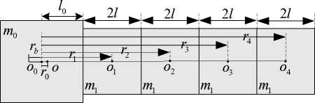
Figure 5. Mass distribution and structure of the asymmetric satellite.
Because the solar array of the satellite must be directed to the sun, the angle that the solar array rotates can be written as O = c sin f .
The main body of satellite is a cubic with mass of m 0 , side length of 2 l 0 . The solar array has four pieces, each can be considered as a rigid plant with piece mass of m 1 , side length of2 l .
Position of the mass center of satellite is
Because of the low density of atmosphere, the drag coefficient can be considered as a constant [3]. The aerodynamic moment can be written as:
v K„2
Ma =- ^^V^CD^^p ( v - v 0 ) X v (3.13)
Where, r v p denotes the vector of aerodynamic pressure center.
Location of aerodynamic pressure center is r = - i (3.14)
p 4 1 0 2 + 8 bl |cos °
-
E. Moment of Solar Radiate Pressure
The moment caused by solar radiate pressure can be written as [3]:
v F N v v 2 v c i=1
Where r v p denotes the vector of solar pressure center of ith surface that is open to the sun, r v 0 denotes the mass center of the ith surface.
As the same reason discussed in the orbit dynamic model, the moment caused by the satellite body can be ignored.
The incoming unit vector of the sunlight can be written vv as - j0 sin a - k0 cos a . Since the solar array is always directed to the sun, the direction of the solar radiate pressure is the same as the direction of the sunlight. Angle of incidence OS = a sin f, unit vector of sunlight vv v n = - j0 sin a - k0cos a , the center of solar radiate pressure is the same as the aerodynamic pressure center.
-
F. Moment of the Earth's Magnetic Field
Distribution of the earth’s magnetic field is as follows [3]:
-
V 2 и v и v и v
B = [-- m- sin i sin( f + to )] i 0 + sin i cos( f + to ) j 0 + i-m cos i g k 0
P 3 P 3 P 3
(3.16)
Where, u m denotes the constant coefficient of the earth's magnetic field, to denotes the argument of perigee.
Assume the magnetic moment of the satellite is along vv x axis, Mmsal = Mmsali , so the perturbation caused by the earth magnetic field can be written as vv v
M m = M msa. x B (3.17)
-
IV. S IMULATION AND A NALYSIS OF U NCONTROLLED A SYMMETRIC S ATELLITE
In this paper, we use the orbital and structural parameters of FY-3 as the simulation model. The technical data are shown in Table I [1]. The results of simulation for this satellite without control are discussed firstly in this section, then some analysis of the unperturbed and perturbed model are presented.
TABLE I. T ECHNICAL D ATA OF FY-3
|
Orbit inclination angle |
i = 98.75 * |
|
Sunlight direction |
a = 10 * |
|
Argument of perigee |
to = 0 * |
|
Time past ascending node |
13:50 |
|
Initial true anomaly |
f , = 0 * |
|
Initial mean anomaly |
M о = 0 * |
|
Drag coefficient |
C d = 2.2 |
|
Semi-major axis |
a = 7,210km |
|
Initial velocity |
V 0 = 7.446km/ s |
|
Orbit altitude |
h=836km |
|
Moment of momentum |
L = 1.287 x 10 14 kg g m 2Z s |
|
Eccentricity of the orbit |
e=0.0015 |
|
Mass of satellite main body |
m 0 = 2,300kg |
|
Solar array (4 in all) |
4 m 1 =100kg |
|
Moment of magnetic momentum |
Mm^ = 0.3 |
|
Side length of satellite body |
2 1 о = 4m |
|
Size of one piece of solar array |
2 1 x b = 1.5m x 3m |
|
Center of satellite body |
r = 0.4166m |
time(s) x 105
Figure 6. Variation of orbital elements with time
|
10 5 фх 0 0.1 0 -0.1 0.1 0 -0.1 |
Attitude Angle |
|||||||||
|
00 |
.2 0 |
.4 0 |
.6 0 |
.8 tim |
11 e(s) |
.2 1 |
.4 1 |
.6 1 |
.8 2 x 10⁵ |
|
|
(WV\ |
'Vaa |
wv |
Дахх |
AW\ |
Uw |
^VW\ |
||||
|
0 0.2 0.4 0.6 0.8 1 1.2 1.4 1.6 1.8 2 time(s) x 105 |
||||||||||
|
^Лу^Г |
Л ^ fi л |
Л А А Л |
ЛллЛ |
мм |
гш |
|||||
|
l/ |
||||||||||
|
0 0.2 0.4 0.6 0.8 1 1.2 1.4 1.6 1.8 2 time(s) x 105 |
||||||||||
Figure 7. Variation of attitude angles with time
-
A. Simulation Results of Uncontrolled Asymmetric Satellite
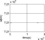
Fig. 6 shows the variation of orbital elements with time in 30 orbit periods. Because the orbit of FY-3 is a nearcircular polar orbit, the altitude of orbit is relatively high, and the surface is not large enough, the influence of the disturbance forces will not be significant. The simulation results also prove this.
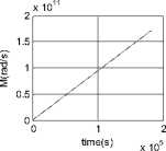
Fig.7 and Fig.8 show the variation of attitude angles and velocities in 30 orbit periods respectively. By estimating all the perturbation moments of asymmetric satellite, the moment of gravity is much larger than the other perturbations. Just like a pendulum, it serves as a stabilizing moment, the rotations around y and z axis can be stabilized. But the rotation around x axis is parallel with the gravity moment, which is not stabilized by the moment of gravity. So the curves corresponding to y and z axis fluctuate around zero, however, the angle around x axis increases rapidly with time due to the accumulation of the moment along x axis.
|
1.5 1.5 1.5 1.5 1.5 |
x 10 'Vly/*v,1 01 |
time(s) x 105
time(s)
x 105
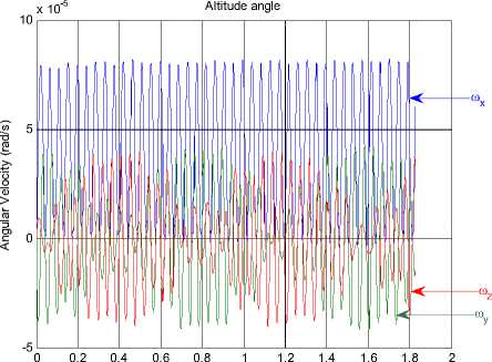
Figure 8. Variation of attitude angular velocities
-
B. Analysis of Unperturbed Asymmetric Satellite
From the simulation in the last section, we can get the conclusion that the disturbance force is insignificant in the orbit dynamic model if the time is not long. We will analyze the attitude dynamic model only in this section; ignore its coupling with the orbit dynamic model.
The following notations are used for simplicity.
Gx = Ix ®x , G = I v® , Gz = Iz ®z x xx y yy z zz
We ignore all the perturbation moments. Since the mass and the moments of inertia of solar array are relatively small when compared with the main body of the satellite, we ignore it either, and then the dynamic equations can be simplified as [5]:
G x
G y
G z
[ 1
к 2

^^^^^^»
— I GG
I xz
1 z У
(4.1)
From the equation (4.1), we have
G = ^r( G x G x + G y G , + G z( G z ) = 0 (4.2)
G
Where, G = .I Gx 2 + G 22 + Gz 2 .
xyz
Integrate equation (4.2), we can get
G r 2 + Gx + Gz 2 = G 2 = const (4.3)
xyz
Equ. (4.3) means that for the variables in (4.1), the phase space of the system can be regarded as a foliation of invariant manifolds
5 2 ( G ) = {( Gx , G y , G z ) | G ^ + G y + G ^ = G 2 } (4.4)
The total angular moment G is a constant. From Equ (4.1), it can be deduced that there are six equilibriums located at the intersections of the body frame axes with the sphere of Equ. (4.4). Two of them located at the y axis are unstable, the other four are stable. The solution to the four asymptotic trajectories is:
Gx = (-1) [( k - 1)/2] G *
sec h ( n 2 t )
G y = (-1) k - 1 G * tanh( n 2 1 )
(4.5)
Gz = (-1) [ k /2] G *
sec h ( n 2 t )
x 104
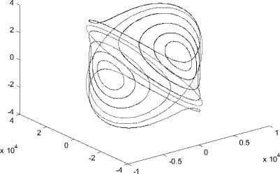
Figure 9. Phase trajectories of unperturbed asymmetric satellite
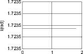
From Fig.9 we can see that all the trajectories of the unperturbed asymmetric satellite are closed curves. This means that the dynamic equations of the unperturbed asymmetric satellite are stable, and the solutions are periodic.
-
C. Analysis of Perturbed Asymmetric Satellite
Since the disturbance forces are not significant in the orbit dynamic model, we will analyze the attitude dynamic model only in this section. We will use the simulation result to discuss the chaotic property of the attitude dynamic model in this section.
Lyapunov Index which is used to analyze the chaotic characters of dynamic equation is defined as follows:
LE = lim-ln
• t ||^ (0)||
(4.6)
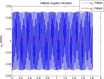
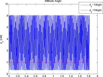
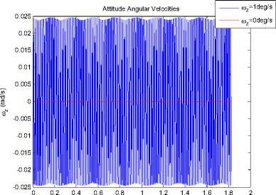
We choose the initial conditions of 9 = 9, = 9 = 0 o , xyz
-
x y z xyz
®x = ®y = ®z = 1 o / s . After 30 periods, variation of each attitude angles and angular velocities of the satellites can be seen from Fig.10 to Fig.15.
The numeric integration reveals that the three Lyapunov indexes as follows:
LE 6 x > 0, LE 6 y = LEez = 0
Since the Lyapunov index of 9x > 0, the error of 9x caused by the errors will increase with time, which is the character of chaotic system. This result is the same as the analysis mentioned above.
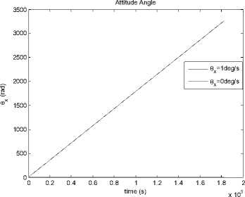
Figure 10. Variation of attitude angle θx with time.
time (s) x 105
Figure 14. Variation of angular velocity ωy with time.
time (s)
x 105
Figure 11. Variation of attitude angle θy with time.
time (s) x 105
Figure 15. Variation of angular velocity ωz with time.
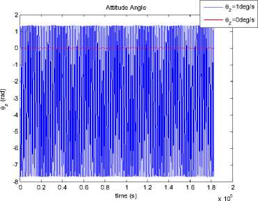
Figure 12. Variation of attitude angle θz with time.
V. O RBIT C ONTROLLER D ESIGN
The orbit dynamic model can be written as Equ. (2.1).
The desired dynamic process of the orbit is as follows:
&= _щ.
rd = 2 rd rd2
(5.1)
We choose the control force as follows:
V
R c
- K15$ - K03$+
^gm Vo r2 r
^m V o
2 r d rd
ˆ
R g
у у
- R a - R S
(5.2)
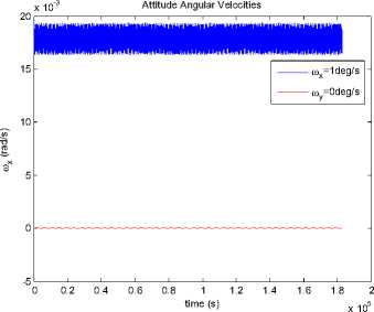
Figure 13. Variation of angular velocity ωx with time.
Where, K0 and K1 are the coefficient matrices for the ˆˆ desired dynamic model of controlled system, Rg , Ra , ˆ and RS are the estimated disturbance forces caused by Earth Non-Sphericity, aerodynamics, and solar radiate pressure. Assume the orbit controller can provide a maximum control force of 20N .
Then the error dynamic process of the controlled orbit dynamic model can be written as follows:
In this paper, we choose
K 0 = diag (2,2, 2) , K 1 = diag (2, 2, 2) ,
So poles of every channel of the controlled system are placed at p = 1 ± j .
Since the disturbance forces do not significantly influence the orbit dynamic model compared with the attitude dynamic model, the estimation of control forces need the attitude of the satellite, and the coupling of orbit dynamic model and attitude dynamic model need to be considered, we will test the property of this controller together with the attitude controller, in the next section.
Control Moments
-
VI. A TTITUDE C ONTROLLER D ESIGN
In this paper, we use the feedback linearization method
-
[2] to design the controller. First we denote
q = Q Q y Q z ] T (6.1)
We choose the control moment as
-1
0 1000 2000 3000 4000 5000 6000 7000
x 10-4
time (s)
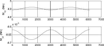
Figure 17. Control moments
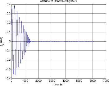
Attitude of Uncontrolled System
MM c = i ( & - к , q - к о q ) -
2h2
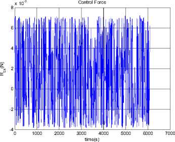
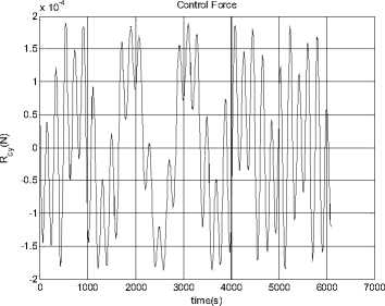
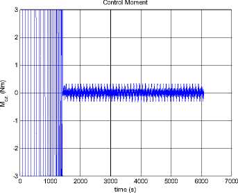
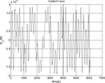
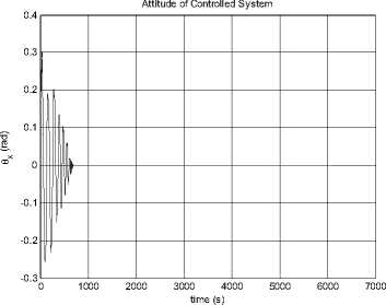
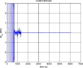
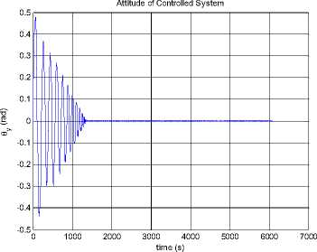
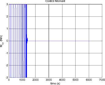
--- P 2h2 —2"Persia. 9cos Qsin p(1 + ecos f )2to p2z Iztoz cos y sin y - Iytoy cosy cos y f Ixtox cos y cos y + Iztoz siny -Iytoy sin y - Ixtox cos y sin y toytoz(Iy-Iz ) toztox (Iz-Ix ) toxtoy(IX-Iy ) z\ z\ z\ z\ - Mg - Ma - Ms - Mm (5.2) Where, K0 and K1 are the coefficient matrices for the desired dynamic model of controlled system, qd is the desired attitude angle vector, <%> = q - qd is the angle error vector, M , Mˆ , Mˆ , Mˆ are the estimates of moments ga sm caused by gravity, aerodynamics, solar radiate pressure, and the earth's magnetic field, respectively. Assume the maximum moment can be provided by attitude controller is 3Ngm . In this paper, we choose K0 = diag(2,2,2), K 1 = diag(2,2,2), So poles of every channel of the controlled system are placed at p = 1± j . We consider the simulation in two conditions as follows. 0.8 0.6 0.4 0.2 -0.2 -0.4 -0.6 -0.8 -1 0 1000 2000 3000 4000 5000 6000 7000 time (s) Figure 18. Attitude angles From Fig. 16, we can get the conclusion that the orbit controller can control the orbit very well, and the control force is not significant. This is similar to the traditional symmetric satellite. In Fig.17 and Fig.18, the attitude can be controlled very well. Fig. 17 shows that the control moments remain small, M and M fluctuate, M remains zero. The yz x attitude of the satellite remains zero. The controller can stabilize the attitude of the asymmetric satellite. Section 4 has indicated that the model is chaotic, i.e. it is sensitive to the initial value. In the next half part of this section, we will test the controller when the system has a small initial error. xyz x yz Figure 16. Control Forces Figure 19. Control Force Rcx Figure 20. Control Force Rcy Figure 24. Control moment Mz Figure 21. Control Force Rcz Figure 25. Attitude angle θx Figure 22. Control moment Mx Figure 26. Attitude angle θy Figure 23. Control moment My Figure 27. Attitude angle θz From Fig.25 to Fig.27, the error of the small initial attitude velocities has caused chaos in the system. That can be inferred more obviously from the control moments shown in Fig.22 to Fig.24, the control moments jump from positive maximum value to negative ones frequently at the beginning of the control process. The controller works as a compensator to try to avoid the chaos [5]. The chaos along the y axis is a little fiercer than other two directions. In Fig.24, corresponding control moment even fluctuates after the system has become stable. With increase of error of attitude, orbit control forces fluctuate more rapidly. This is because of the coupling between orbit dynamic model and attitude dynamic model. VII. CONCLUSIONS AND FUTURE WORK The feedback linearization method not only works well to exempt perturbation moments in the attitude control problem, like the traditional linear controller, but also can work far from its equilibrium. The simulation in Section 5 shows that it works well even the system becomes chaotic. Despite the controller designed can work well for the dynamic system, factors such as energy consumption in the control process must be taken into consideration in the future. We can see this factor from Fig.15, in which the control moment along y axis is influenced by the chaos a bit more than the other two. The energy consumed is enormous in the practical circumstances. Chaos can also be used in the control process, not just try to exempt it, some recent work reveals that chaos can be helpful while dealt properly. The results show that the control moments jump from positive to negative maximum frequently, especially at the beginning, when the system becomes chaotic. To solve this problem, other control methods, such as robust control, can be used after the feedback linearization has been applied. The orbit dynamic model of asymmetric satellites is almost the same as symmetric ones, but the attitude dynamic model is completely different, so we can apply orbit control strategy of symmetric satellites to asymmetric ones, but we have to design the control strategy for its attitude dynamic model. ACKNOWLEDGMENT The authors wish to thank all the reviewers for their valuable comments and suggestions that improved the quality of this paper.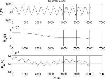
References Orbit and Attitude Control of Asymmetric Satellites in Polar Near-Circular Orbit
- FY-3, http://baike.baidu.com/view/931210.htm.
- J-J. E. Slotine, and W. Li, Applied nonlinear control, MIT Press, Oct. 2004.
- Y. Z. Liu, Attitude dynamics of spacecrafts (Chinese), National Defense Industrial Press, Beijing, Dec. 1995.
- X. N. Xi, and W, Wang, Fundamentals of near-earth spacecraft orbit (Chinese), National University of Defense Technology Press, Changsha, Apr. 2003.
- M. Inarrea, V. Lanchares, V. M. Rothos, and J. P. Salas, “Chaotic Rotations of an Asymmetric Body with Time-Dependent Moments of Inertia and Viscous Drag”, International Journal of Bifurcation and Chaos, Vol. 13, No. 2, World Scientific Publishing Company, 2003, pp. 393-409.
