Особенности формирования мелкомасштабных волновых возмущений во время резкого сжатия магнитосферы

2009 event. Using synchronous satellite and ground observations, we study spatial-temporal characteristics of the pulsations to determine causes of their generation.

2.    EXPERIMENTAL DATA

Characteristics of the disturbances in the interplanetary medium and in the magnetosphere are analyzed using ACE, WIND, CLUSTER, THEMIS satellite data in GSM coordinates as well as data from ground geomagnetic stations under the following projects: CPMN , THEMIS (http: //, IMAGE , and Greenland coast chain ( . Table 1 and Table 2 list the coordinates of the satellites and ground stations respectively.

Table 1

Satellite coordinates in the interplanetary medium and in the magnetosphere

Satellite	Time, UT	Coordinates
		X GSM , R e	Y GSM , R e	Z GSM , R e
ACE	23:48	238.94	–23.12	–34.58
WIND	23:48	230.15	79.99	55.58
CLUSTER 4	00:50	7.84	–2.19	–0.87
CLUSTER 2	00:50	7.57	–3.10	–0.10
CLUSTER 3	00:50	5.47	–1.07	0.85
THEMIS E	00:50	–6.28	7.79	1.77
THEMIS D	00:50	–7.17	7.69	2.01

Table 2

Coordinates of geophysical stations

Station	Abbreviation	Geographic		Magnetic		MLT midnight in UT
		Lat, deg	Long, deg	Lat, deg	Long, deg
Ф'=69–73°
Bear Island	BJN	74.50	19.20	71.29	109.18	21:08
isl. Kotelny	KTN	76.0	137.9	70.01	201.10	15:51
Barrow	BRW	71.32	203.38	70.29	253.46	12:02
Kaktovik	KAKO	70.13	216.35	71.08	264.22	11:07
Inuvik	INUV	68.41	226.23	71.23	275.09	10:17
Yellowknife	YKC	62.40	245.50	69.58	299.56	9:09
Cape Dorset	CDRT	64.2	283.4	73.5	1.7	04:55
Sondre Stromfjord	STF	67.02	309.28	73.16	41.74	02:17
Ф'=63–66°
Dønna	DON	66.11	12.50	63.38	95.23	21:59
Tixie	TIX	71.6	128.9	65.69	196.98	16:04
Chokurdakh	CHD	70.6	147.9	64.68	212.18	15:09
Kiana	KIAN	66.97	199.56	65.13	253.47	12:02
CIGO College	CIGO	64.87	212.14	65.06	265.11	11:06
White Horse	WHIT	61.01	224.78	63.67	279.14	10:01
La Ronge	LARG	55.15	254.74	62.69	317.59	07:27
Sanikiluaq	SNKQ	56.536	280.77	66.45	356.99	05:12
Nain	NAIN	56.4	298.3	64.65	22.08	03:40
Narsarsuaq	NRSQ	61.16	314.56	66.31	43.91	02:06

3.    OBSERVATIONAL RESULTS 3.1    Interplanetary medium parameters

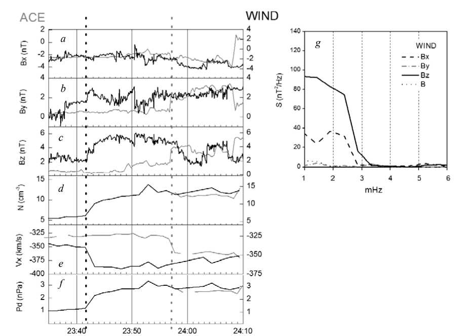
Figure 1 presents the solar wind parameter data from the WIND (black lines, right scale) and ACE (gray lines, left scale) satellites.

From top to bottom, variations of IMF B x , B y , B z components (Figure 1, a – c ), SW density (N), SW velocity ( V x ), and SW dynamic pressure ( P d ) (Figure 1, d – f ) are shown. Dashed lines indicate registration moments of the IPS front by these satellites. The WIND satellite, located closer to the magnetosphere (see Table 1), recorded IPS about 15 minutes earlier than the ACE satellite. Consequently, the IPS front was inclined to the Earth–Sun line in the Z_GSM=0 plane. According to data from both the satellites, the passage of the IPS front was not followed by a change of sign of the IMF components: B x was negative, B y and B z were positive. In general, variations of interplanetary medium parameters are typical for IPS. The WIND satellite observed irregular long-period IMF variations. In the oscillation spectrum (Figure 1, g ), calculated for 23:35–23:59 UT, there is a maximum at a frequency of 2 mHz in IMF B x . In the spectrum of oscillations in IMF B z , such a maximum is not observed, but there is a sharp intensity decrease at a frequency above 2.3 mHz (similar to IMF B_x ).

Figure 2 shows the satellite location in the ZGSM=0 plane in the interplanetary medium (a, ACE, WIND) and in the magnetosphere (b, CLUSTER (Cl) 2, 3, 4, THEMIS (Th) D and E). Using the multi-satellite method mentioned in [Schwarth, 1998], we have defined the normal components, azimuthal (Az) and meridional (Mrd) angles of the IPS front inclination. Values of these parameters are given in Table 3. From this table it follows that in the interplanetary medium the azimuthal angle of inclination of the front is ~13.8° (it is counted counterclockwise from the negative X axis in the GSM-coordinate system), and in the magnetosphere it is ~34.1°. The meridional angle varies from ~0.2° in the interplanetary medium up to ~3° in the magnetosphere. Figure 2, a, b is the schematic of the front orientation in the interplanetary medium and in the magnetosphere.

3.2    Magnetospheric and ground observations

Figure 3, a , b illustrates variations of the geomagnetic field H component for the April 24, 2009 event as derived from data from high-latitude stations located at close latitudes in different longitudinal sectors. It is seen that at 00:50–01:20 UT at auroral latitudes in the noon (9–10 MLT, KTN, TIX, CHD) and evening (20 MLT, STF, NRSQ) sectors, 8–9 min pulsations were registered. The maximum pulsation amplitude of ~50 nT was observed at the KTN station ( Φ '=71°). In the 13–14 MLT sector at latitudes 63–66°, short-period pulsations (5 min) were recorded (Figure 3, b ).

Phase delays of SI onsets at the stations located in adjacent MLT sectors point to azimuthal propagation of the shock front to the west (gray arrow) and to the east (black one). Propagation in opposite directions was observed in the 15–17 MLT sector, where the IPS shock first contacted with the magnetopause. The azimutha propagation velocities estimated by delays between the neighboring stations were: YKC-INUV~15 km/s, INUV-KAKO~11 km/s, KAKO-BRW~9 km/s, YKC-CDRT~17 km/s (Figure 3, a ), WHIT-CIGO~11 km/s, CIGO-KIAN~18 km/s, KIAN-CHD ~12.5 km/s, CHD-TIX~12 km/s, and LARG-SNKQ ~15 km/s (Figure 3, b ).

ит

Figure. 1 . Interplanetary medium parameter data aboard the WIND (black lines, right scale) and ACE (gray lines, left scale) satellites. From top to bottom are the IMF B x , B y , B z components ( a – c ), SW density, velocity, and dynamic pressure ( d – f ), and IMF spectra ( g ) in the interval 23:35–23:59 UT. Time moments when the IPS front was registered by these satellites (dashed lines)

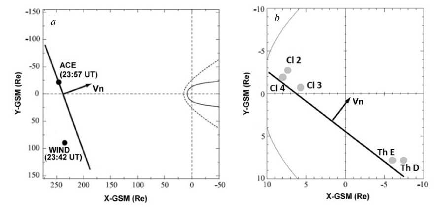
Figure. 2 . Satellite location in the GSM XY plane in the interplanetary medium (ACE, WIND) ( a ) and in the magnetosphere (CLUSTER (Cl) 2, 3, 4, THEMIS (Th) D and E) ( b ). The orientation of the IPS shock front and compression wave front (solid lines)

Table 3

Components of normal, azimuthal, and meridional angles of inclination of the shock front in the interplanetary medium and in the magnetosphere

Satellite	N x	N y	N z	Az ,	Mrd ,°
ACE-WIND-Cl 4-Th D (sw)	–0.9710	–0.2390	0.0037	13.8261	0.2115
Cl 4-Cl 3-Th E-Th D (m/sphere)	–0.8265	–0.5605	0.0532	34.1448	3.0468

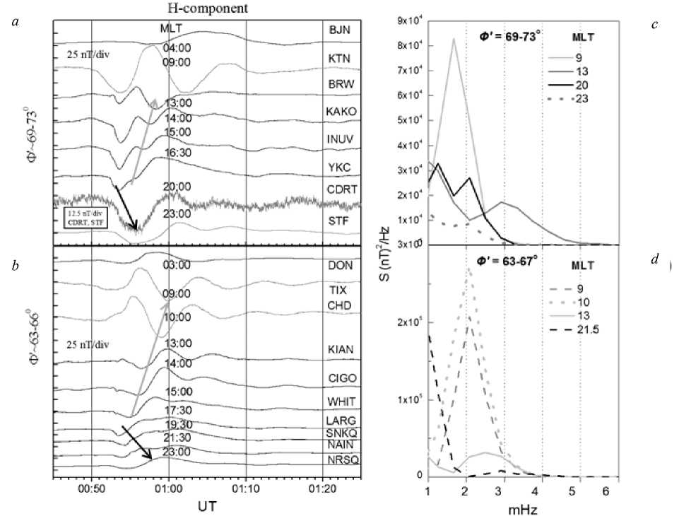
Figure. 3 .Variations of the geomagnetic field H component according to data from the stations extended along Ф´=69–73° ( a ) and Ф´=63–66° ( b ) latitudes, frequency spectra of variations ( c , d ) in the interval 00:45–01:25 UT. Azimuthal propagation to the west (gray arrow) and to the east (black arrow)

Thus, there is a tendency for azimuthal velocity decrease with distance from the sector, where the initial contact occurred. Such velocity dynamics is consistent with the results of other studies.

Figure 3, c , d shows the frequency spectra of variations at the stations presented in Figure 3, a , b in the interval 00:45–01:25 UT. The spectra are demonstrated to begin from 1 mHz to exclude the lower-frequency variations associated with magnetospheric compression from consideration. It is seen that the spectra have pronounced maxima in the noon sector at frequencies of ~1.7 mHz (Figure 3, c ) and 2.1 mHz (Figure 3, d ). In the evening sector (Figure 3, c , 20–23 MLT), there are maxima at frequencies of 1.2 and 2.1 mHz, i.e. at frequencies close to the oscillation frequency at the noon sector, but with a much lower amplitude (Figure 3, a , the CDRT and STF stations).

Figure 4, а depicts variations of the magnetic field total intensity aboard the magnetosphere satellites (Figure 2, b ). Figure 4, b illustrates the V x -component of plasma flow velocity aboard the same satellites. Both the magnetic field and the plasma flow velocity are shown for a short interval of 15 minutes (00:50– 01:05 UT). The moments of the sharp change of the

magnetic field correspond to the passage of the shock front in the vicinity of the satellites (dashed lines). Numbers indicate the delays of registration of the shock front in seconds aboard the satellites relative to that at the Cl 4 satellite. We use these delays and coordinates of the satellites to estimate the front propagation velocity in the interplanetary medium and in the magnetosphere. It is seen that the compression effect is most pronounced in the dayside magnetosphere. The analysis of plasma flow velocities has revealed the presence of wave disturbances aboard the Cl 3 and Th D satellites similar to those ones ob-

served on the ground (Figure 4, b , Figure 3, a , b ). The moments of registration of the minimum plasma flow velocities corresponding to the earthward motion of plasma are marked with dashed lines in Figure 4, b . For these moments, we have calculated the front propagation velocities ( V _n), which are shown in the first row of Table 4.

V n velocities are estimated by the formula

V n =

V d N d N

- V N u )

- N u J

n ,

where V d , N d are the downstream velocity and density,

Table 4

Shock front propagation velocities and Alfvén velocities as inferred from satellite observations

V , km/s	WIND	Cl 4	Cl 2	Cl 3	Th E	Th D
V n	399	47.6	74.8	53.1	58.9	48.5
V ≈2 L / T	–	1204.4	936.8	1018	2750	2942.8

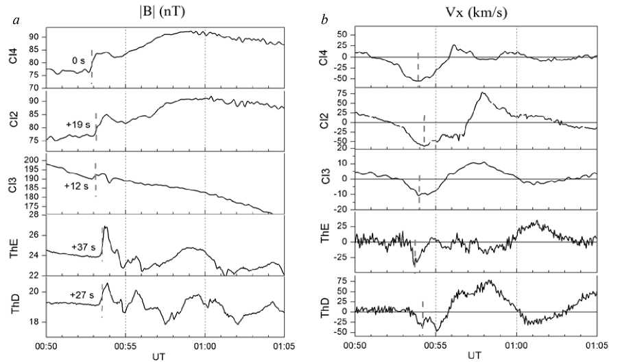
Figure. 4 . Magnetic field total intensity ( a ) and V_x -component of plasma flow velocity ( b ) aboard the magnetosphere satellites in the interval 00:50–01:05 UT. Time moments correspond to the passage of the shock front in the vicinity of the satellites (dashed lines). The delays of registration of the shock front in seconds relative to the Cl 4 satellite (numbers)

V u , N u are the upstream velocity and density, n is the normal to the front.

The second row of this table lists the velocity values derived from the formula

V ≈ 2 _T ^L , (2) where L is the field line length, T is the oscillations period.

The field line length is estimated by the Tsyganenko model (T96). Table 4 shows that the front velocity ( V n ) is much less than the Alfvén velocity in the outer magnetosphere ( V ≈2 L / T ) as inferred from satellite measurements. However, V n is comparable with the front propagation velocities obtained in [Kim et al., 2012] and, probably, corresponds to the gradual compression of the magnetosphere by the IPS front.

Estimating the front propagation velocity, we suppose that the front propagates in the Z GSM =0 plane. It is possible that propagation also occurs in the meridional plane because the meridional angle of the front inclination is nonzero, although much less than the azimuth angle.

Figure 5, a shows components of the magnetic (left scale, black lines) and electric fields (right scale, gray lines) aboard the Cl 3 satellite. Both the magnetic field and the electric field are in magnetic field-aligned (MFA)

coordinates and are filtered in a range 400–1000 s. In the MFA coordinates, the B o component (the field-aligned component) is directed along the magnetic field line, B a (azimuthal component) is directed to the east, and B r completes the right-handed triplet vectors. Figure 5, b and c depict the magnetic and electric components of compressional, poloidal, and toroidal modes respectively. Figure 5, d shows the phase difference between the electric and magnetic fields for different modes. Referring to Figure 5, b , d , the most regular oscillations were recorded in the magnetic and electric components of the toroidal mode, and only between them the phase shift accounted for 90°, i.e. there was a toroidal standing wave.

In the spectra of the magnetic and electric fields (see Figure 5, e , f ), calculated by unfiltered Cl 3 data, there are noticeable peaks at a frequency of 1.7 mHz in the B _a и E r components. The Th D satellite (Figure 5, g , h ) observed a broad spectral maximum at frequencies 2.1–2.5 mHz. In the Cl 3 spectra, there are also maxima at 2.1 mHz in the B _r and E _a components, but with much lower amplitude compared to the maxima at 1.7 mHz.

Figure 5, i , j , k illustrate the spectra of magnetic field oscillations recorded by the Cl 4, Cl 2 and Th E satellites respectively. Figure 5, l shows the spectrum of electric field oscillations aboard the Th E satellite.

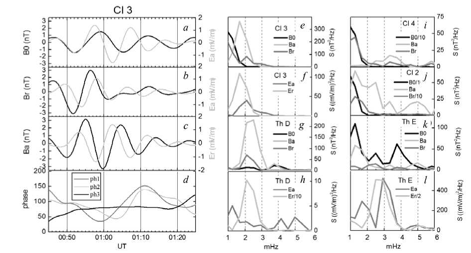
Figure. 5 . B o , B r , B a components of the magnetic field (black line) and E r , E a components of the electric field (gray line) in the magnetosphere aboard the Cl 3 satellite. Magnetic and electric components of compression ( a ), poloidal ( b ), toroidal ( c ) modes and the phase shift between them ( d ), the frequency spectra of the variations of magnetic and electric fields aboard Cl 3 ( e , f ), Th D ( g , h ), Cl 4 ( i ), Cl 2 ( j ), and Th E ( k , l ) at 00:45–01:25 UT.

As follows from the spectra shown in Figure 5, e – k , a feature of the oscillations recorded by the Cl 3 and Th D satellites is maxima in the B a and E r components at frequencies of 1.7 and 2.1 mHz. At Cl 2 and Cl 4 (Figure 5, i , j ), oscillations with such frequencies were not observed. The Th E satellite, which was located ~0.9 R e along the X coordinate closer to Earth than Th D, recorded a powerful peak in the E r component at higher frequencies (2.5–2.9 mHz) despite the absence of maximum in the B a component. The predominant excitation of oscillations in these components is typical for the toroidal mode. Thus, the toroidal mode oscillations prevail in the pre-noon and evening sectors.

Figure 6 presents hodographs of plasma velocity ( V xy ) and magnetic field ( B xy ) in the XY plain as inferred from satellite (Cl 3 in Figure 6, a , Th D in Figure 6, e ) and ground (Figure 6, b , c , d , f , g , h ) observations in the pre-noon and evening sectors between 00:53–01:03 UT.

The Figure indicates that the pulsations have an elliptical polarization, i.e. in the pre-noon magnetosphere (Cl 3, Figure 6, a) the counterclockwise rotation was observed; and in the evening sector, the clockwise rotation (Th D, Figure 6, e). The comparison of pulsations in both the sectors shows their similarity. The ground-based stations observed latitudinal changes of polarization in the pre-noon sector. The clockwise rotation occurred at a latitude of 70° (KTN, Figure 6, b); and the counterclockwise rotation, at a latitude of 66° (TIX, CHD, Figure 6, c, d). In the evening sector at 64–67° latitudes, the oscillations are polarized clockwise, as derived from both satellite and ground data. The opposite direction (counterclockwise and clockwise) and inclination of polarization ellipses on opposite sides of the noon meridian are typical for sudden impulses and their associated geomagnetic pulsations. They reflect propagation of the impulses and pulsations in different directions from the noon meridian, as is assumed in [Takeuchi et al., 2002].

The latitudinal change of polarization in the prenoon sector probably reflects the resonant nature of oscillations, but this feature can be explained by the vortex motion, as is shown in [Takeuchi et al., 2000] for the global vortices excited during SI.

4.    DISCUSSION 4.1    Spatially localized variations of the electromagnetic field and plasma parameters

Besides the global geomagnetic field disturbances caused by ionospheric current systems during sudden impulses [Araki, 1994], a comparatively local quasi-periodic changes of the magnetic field may occur. Hodographs of these disturbances both from magnetospheric and ground-based (ionospheric) observations are vortices. Such vortices during SI are observed rather rarely [Yahnin et al., 1995], perhaps, due to the following reasons: a) the IPS front should be inclined in the ecliptic plane (as in this event), which leads to asymmetric compression of the magnetosphere, and hence to geomagnetic variations asymmetric relative to the noon [Vorobyev, 2000]; b) it is difficult to detect such vortex disturbances because of their small scales.

In [Shi et al., 2014], the wave disturbance in the night plasma sheet in the event considered has been analyzed. The authors identified the resonant nature of the disturbance and suggested that it was caused by the vortex interaction with a resonant L-shell. The vortex appeared during the contact of IPS front with the magnetopause and propagated deep into the magnetosphere.

Taking into account their results and the polarization of the oscillations (Figure 6), we can assume that the

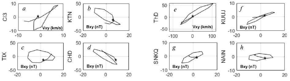
Figure. 6 . Hodographs of plasma flow velocity ( a , e ) inferred from satellite data and the magnetic field ( b , c , d , f, g , h ) from ground data at 00:53–01:03 UT

pulsations in our event in both the sectors were generated by vortices. For the analysis of source of the vortices in this event, we have plotted a distribution of horizontal velocities of the compression wave front (V1, gray arrows) and the plasma flow (V2, black arrows) at 00:55 UT (Figure 7). It is seen that aboard the Cl 3 satellite the velocities differed greatly in magnitude (projection of V2 to V1 is indicated by the outline arrow), i. e. intense shear flows were recorded. The Th D and Th E satellites observed a similar velocity difference but with lower magnitude.

The insets a and b in Figure 7 illustrate the dynamics of the horizontal velocity vector of the plasma flow as derived from the Cl 3 and Th D satellite data respectively. At 00:54–00:58 UT, the Cl 3 satellite observed velocity vector rotation, followed by positive velocity values corresponding to the westward plasma flow and then by negative velocity values corresponding to the eastward flow. The Th D satellite observed the velocity vector rotation between 00:56–00:59 UT and then oppositely directed flows, as aboard Cl 3. Keiling et al. [Keiling et al., 2009] present a scheme explaining the dynamics of plasma velocity vector depending on which part of the vortex crosses the satellite and on the direction of vortex rotation (Figure 7 therein). According to this scheme, the dynamics of velocity vectors corresponds to vortices of opposite directions, i.e. clockwise rotation was registered by Cl 3; and counterclockwise one, by Th D. Such pattern coincides with the polarization of oscillations in Figure 6, a and e .

Shi et al. [2014] discussed the possible mechanisms of wave disturbance generation in the night plasma sheet in this event and recognized the interaction of vortex with the resonant field line as the most probable mechanism. This is also supported by the results of the MHD simulation they carried out.

Moretto et al. [2002], when considering the vortical disturbances in the dayside magnetosphere, have assumed that the disturbances are caused by wave disturbances at the magnetopause, which make plasma move radially into the magnetosphere and then plasma is reflected outward from the inner boundary, which may be the plasmapause.

But how then to explain the oscillations in the evening sector where it is difficult to find an inner boundary? Such a boundary could be a plasmaspheric plume; how- ever, this phenomenon occurs under disturbed conditions, whereas our event happened under quiet conditions. This fact testifies that the oscillations in this event, especially in the evening sector, were caused by the vortex that formed on the evening flank of the magnetosphere and then started to move to the night side.

The results of our analysis are indicative of the relationship of the wave disturbances on the night side, which were considered by Shi et al. [2014], with disturbances in the daytime sector. The location of wave disturbances in the magnetosphere at different radial distances, i.e. X ~5.6 R _e in the noon sector and X ~ –7.2 R _e in the evening sector, is consistent with the inclination of the IPS front in the ecliptic plane. It is assumed that the compression wave front propagating in the magnetosphere with the average velocity V n ~56.5 km/s caused the vortical disturbances in the regions, where the front propagation and plasma flow velocities differed most greatly in magnitude. Apparently, the inclination of the front in the ecliptic plane had crucial importance in the formation of vortical disturbances in this event.

4.2    Mechanism of vortices

The dependence of frequency of excited oscillations on latitude (Figure 3) and the predominance of oscillation amplitude in the toroidal component (Figure 5) point to the resonant excitation mechanism of pulsations in this event. At the same time, the oscillation spectra in the interplanetary medium and in the magnetosphere have a common peak with a central frequency of about 2 mHz. Thus, we cannot exclude the possibility of penetration of the waves from the interplanetary medium.

The penetration of oscillations in the Pc5 range from the interplanetary medium into the magnetosphere was considered in [Kepko et al., 2002; Kepko, Spence, 2003]. In [Kepko et al., 2002; Kepko, Spence, 2003], when analyzing a series of geomagnetic pulsations caused by P d variations, it has been found that discrete frequencies (1.3, 1.9, 2.6, and 3.4 mHz) of intramagne-tospheric resonances are observed in SW density variations and probably indicate the existence of structures of certain sizes in the interplanetary medium (it is necessary to note that in our event the oscillation frequency is close to one of the intramagnetospheric resonance frequencies (1.9 mHz)).

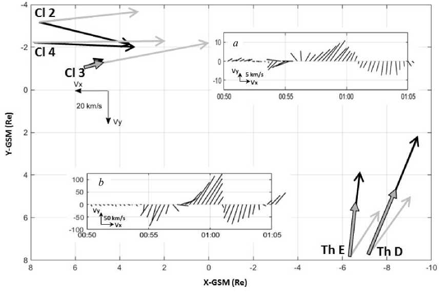
Figure. 7 . Spatial distribution of propagation velocities of compression wave front (gray arrows) and plasma flow (black arrows) at 00:55 UT. The insets ( a ) and ( b ) illustrate the dynamics of the velocity vector of plasma flow aboard the Cl 3 and Th D satellites respectively

The P d variations [Kepko et al., 2002; Kepko, Spence, 2003], Kelvin–Helmholtz instability and combined instability of Kelvin–Helmholtz–Rayleigh–Taylor [Mishin, 1993], which act as an amplifier of ULF waves incident on the magnetopause, have been proposed as the mechanisms of direct penetration of Pc5 waves from the interplanetary medium. Moreover, in [Kessel et al., 2004], it has been established that wave activity amplifies in the magnetosheath by a factor of 10, compared to the interplanetary medium.

The P d variations and above instabilities are unlikely to be the cause of the vortices in this event because the pulsations they generated would have been recorded globally and would have manifested themselves in changes of the total magnetic field intensity aboard the satellites. As follows from Figure 4, a , the satellites did not record magnetic field changes with a period 8–9 min, but the Th D and Th E satellites observed 1–1.5 min variations, which might reveal global magnetospheric oscillations. In [Samsonov, 2014], the 2.6 min pulsations immediately after SI in a geostationary orbit were interpreted as global magnetospheric oscillations. It is well known that toroidal Alfvén waves and global compression waves in the magnetosphere can be excited simultaneously. So, in [Parkhomov et al., 1998], it has been found that the sharp P _d decrease manifested itself in the generation of pulsations of two types at frequencies of 2.3 mHz and 6.4 mHz. The authors suggested that the first type with a latitude-independent period is related to the magnetopause oscillations, and pulsations of the second type, whose period depends on latitude, is caused by field line resonances.

It is also known that IMF variations can directly lead to the formation of vortices or ULF waves in the magnetosphere [Nedie et al, 2012; Moiseyev et al, 2014]. In those works, the authors examined pulsations in the magnetosphere and on Earth caused by IMF B z variations. In our event, the waves in the interplanetary medium at almost the same frequency of 2 mHz are most pronounced in the IMF B x and B z components (Figure 1). Thus, the IMF variations specify the frequency of oscillations in this event.

CONCLUSION

• •    Vortical disturbances of the magnetic field and plasma velocity in the magnetosphere in the noon and evening sectors whose positions are consistent with the inclination of the compression wave front have been found.

• •    Oscillations of the electromagnetic field and plasma velocity observed in the vicinity of the vortices are resonant.

• •    The analysis of the distribution of plasma flow velocities and compression wave front propagation in the magnetosphere’s equatorial plane has shown that the vortical disturbances are observed in regions, where the velocities differ in magnitude.

We are grateful to E. Tanskanen for IMAGE project data, to National Space Institute at the Technical University of Denmark (DTU Space) for the Greenland Magnetometer Array data, and to D.J. McComas, R. Lepping, K. Ogilvi, G. Paschmann, and G. Reeves for satellite observation data from CDAWEB. This work was partially supported by the RFBR grants No. 15-45-05090 (MA), grant No. 15-05-05561 (MV) and by the program JSPS Core-to-Core Program, B. Asia-Africa Science Platforms.