Parallel Implementation of a Video-based Vehicle Speed Measurement System for Municipal Roadways

Published Online November 2019 in MECS

For several years, providing safe and secure transportation circumstances have been considered as the basic requirement for the development of industries and increasing social welfare level in developed countries [1]. Nowadays, transportation issues such as environmental pollutions, reduction of energy resources, corporeal and financial damages caused by car accidents and the rapid growth trend of transportation demands - especially during the peak hours of road traffics - have become an unbreakable challenge in all cities around the world [2]. In this regard, Intelligent Transportation Systems (ITS) are defined as the means for collection of tools, facilities, and specializations, such as traffic management and telecommunications technologies in the form of coordinated instruments. ITS have various branches to provide the desired solutions to tackle the mentioned issues [3]. One of the main applications of ITS is the automatic speed measurement. Due to the possible dangers such as vehicle-pedestrians’ accidents, vehicles’ speed control procedure on urban roadways is very important. There are several methods for speed measurement purposes and many systems designed over the time to calculate the passing vehicles’ speeds, like inductive loop detectors, Laser-based (Lidar) and Radarbased systems [4]. Inductive loop detectors are known as widely used instruments, but they suffer from some major problems such as challenging installation and maintenance, short lifetime and road damage [5]. On the other hand, Laser-based and Radar-based systems are more expensive than inductive loop detectors, but they have the advantage of better accuracy [6]. Here, the accuracy is defined as the proximity of a vehicle’s real instantaneous speed and calculated speed. As another type of devices, speed sensors using Digital Image Processing (DIP) have attracted huge interest among researchers in recent years. These systems, which known as vision-based approaches, use the video output of installed road cameras and process them to obtain information about the vehicle’s speed [7]. Vision-based methods can be remarked as alternatives for existing speed measurement systems, i.e. Radar and Laser-based applications, in case they provide acceptable accuracy. Although these approaches suffer from some limitations like high computational cost and some challenges in detecting and tracking vehicles in the video scene, measuring vehicle speeds using DIP has several advantages such as lower cost, easier maintenance, and better expandability.

In this paper, we introduce a parallel implementation of a formerly presented computationally intensive visionbased vehicle speed measurement method [12] to provide a real-time performance by utilizing GPU for parallelization. Experimental results have shown about 55.12% decrease in the execution of the parallelized version compared to the CPU-based approach. It should be noted that some minor changes in vehicle detection and tracking modules have been applied which are thoroughly explained in related sections. The main contributions of our work are summarized below:

• 1)    We developed a parallel implementation of a sequential (CPU-based) speed measurement approach;

• 2)    General analysis and profiling of the method to detect computationally intensive modules with low dependencies to other modules was performed;

• 3)    The effect of parallelization in both kernel and application levels was calculated;

• 4)    We observed that by parallelizing some computationally intensive modules made the method robust against executing in almost realtime applications;

The rest of the paper is organized as follows: we will first explain the definitions and some related works in Section 2. In Section 3, the description of the proposed method which is a parallelized implementation of a speed measurement approach including motion detection, license plate recognition, vehicle tracking, and speed calculation modules is introduced. Experimental results and evaluations are presented in Section 4 and finally, we finish with conclusions in Section 5.

• II.    R elated W orks

In this section, some primary concepts are introduced to provide a better understanding of the speed measurement process and later, some related works are presented and discussed. As a common classification of vision-based speed measurement approaches, two main categories, including motion-based and appearance-based methods are existed [7]. Motion-based approaches do not depend on visual features of the vehicles and instead, require a sequence of frames to detect moving vehicles. Although these methods are able to recognize the depth of the scene, they do not represent vehicles by their visual features and thus, they provide lower computational costs. Appearance-based approaches, on the other hand, need some visual features of the vehicles, e.g. license plate or tail-light, in each frame. As a common manner, vehicle speed measurement algorithms using DIP have a general block diagram as shown in Fig. 1. They come along with some differences in applying algorithms for each part of the scenario which may result in different computational costs and performance. As it can be mentioned, in the first step, the general topographies of moving vehicles in the scene should be detected using various methods such as background subtraction or frame differencing in motion-based, and visual pattern or texture in appearance-based approaches. These features may be existed in the whole or some special regions of vehicles, like the headlights, license plate, etc. In the next step, the previously found features should be tracked among sequential frames to provide the vehicle’s displacement in pixels. Tracking process makes it possible to measure the amount of the moving vehicle’s displacement to provide speed measurement parameters. The final results of this process can be some special parts of the vehicles or the whole vehicle’s shape. Finally, a module to calculate vehicle speed through mapping pixels to meters and frame numbers to seconds is performed. This mapping function should convert the displacement vector ⃗⃗⃗⃗ in the camera’s focal length to the displacement vector ⃗⃗⃗⃗ in real-world metrics.

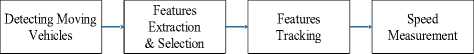
Fig.1. A general block diagram of common vision-based speed measurement methods.

Because of the direct recognition of vehicles in separate frames, these methods are faced with high computational cost and time consumption to provide appropriate accuracy. In this regard, parallelization of such algorithms is an appropriate process to tackle high computational costs by concurrent execution of procedure divisions on various processing units. In recent years, Graphical Processing Units (GPUs) have become significantly powerful tools for parallelization purposes. GPUs, with the help of their abundant number of processing units, are able to provide SIMT (Single Instruction Multiple Threads) parallelization and execute a method in a fraction of time required for the execution of the same method on CPUs.

• A. Background Information

In this sub-section, some important definition of concepts and background information which have been used in the upcoming parts of the paper are presented [811]:

• • Compute Unified Device Architecture (CUDA):

in order to utilize a Graphical Processing Unit as a powerful device to speed up computationally intensive algorithms, CUDA has been developed by NVidia as a great programming tool for parallelization. Before introducing CUDA, the task of GPU programming was tough and the programmer needed to know the main architecture of the GPU. CUDA simplified the implementation of GPU-enabled applications to be rendered on NVidia GPUs. Computationally intensive applications with the lowest possible dependencies are the best candidates for parallelization on CUDA. This environment makes programmers able to distribute the amount of computation in their codes on thousands of cores of their GPU cards and consequently, provide the performance equal to tens of CPUs with much less cost. In CUDA, kernels are referred to data-parallel portions of an application, which contain several threads for parallel execution to be operated on data stored in the GPU’s memory. It should be mentioned that the process of initiating the kernels is done by CPU. For parallelization of an application, these threads should be grouped together to provide warps and blocks of codes. The main challenge for the programmer is to avoid serially execution of threads and provide optimized performance.

• •    Good features: Since selecting appropriate features equivalent to the physical points in ground truth is a difficult process, correct detection of these features is so important in object tracking goals. A “good feature” as it is mentioned in [9], is a region with high-intensity variations in more than one direction, like the areas of texture or corners. In this regard, Good Features to Track [9] is a corner detection approach based on the Harris corner detector which finds the strongest corners in an image and skips the corners below a pre-defined quality. So the output of this function is a number of corners which are appropriate for later tracking that makes the system needless of extracting information from every single corner in an image.

• •    Motion History Image (MHI): MHI is a common vision-based method for detecting moving objects in sequential frames which uses a static image template to understand the location and path of the motion. This technique has some advantages such as insensitivity to silhouette noises, holes, shadows and missing parts, and the ability of implementation in low illumination conditions. In MHI method, the intensity of each pixel in a temporal manner is used for motion representation, and a history of changes at each pixel location is stored for motion detection purposes.

• •    Pyramid version of Kanade-Lucas-Tomasi

(KLT): because the traditional algorithm of KLT only works for small displacements (in the order of one pixel), the pyramid version of this method is used in [10] to overcome the limitation of larger displacement detections. The pyramid version of KLT algorithm picks up a pyramid for each frame, where the image with the main dimensions is placed at the base of the pyramid. In each level, the width and height of the image are reduced by half. The pyramid KLT algorithm begins to find the vector ^⃗ԁ^⃗ of displacement from the last level of the pyramid and uses the results for the initial estimation of ^⃗ԁ^⃗ at the next level. This process continues to reach the base of the pyramid, i.e. the original image .

• •    T-HOG text descriptor: this text descriptor which was first presented in [8], detects a collection of characters by obtaining a gradient histogram of the top, middle and bottom of an image area by the means of the histograms of text regions. These areas have significant and fundamental differences with other non-text regions. Consequently, this method can be used to detect a vehicle’s license plate regions in a video frame for further processes.

• B. Related Works

Due to the numerous benefits of video-based ITS approaches, some different methods for estimating and measuring the speed of vehicles on the roadways are proposed. Most of these techniques use background/foreground segmentation algorithms to detect vehicles and track them in sequential frames to calculate their displacement in a period of time. These approaches follow the steps shown in Fig.1 in most of the cases. In [12], a frame differencing technique to detect moving vehicles is presented that seeks a vehicle’s license plate to extract desired features and track its good features in multiple frames using the pyramid KLT algorithm. The speed measurement average error in this approach was -0.5 km/h and in over 96.0% of cases, measurement errors were inside [-3, +2] km/h range. Similarly, a robust approach presented in [13] used the same vehicle detection technique which considers each vehicle as a blob by the means of the edge detection method and tracks their centroids to calculate the displacements of blobs in a limited time range and measure the vehicles’ speed. In [14], another frame differencing method to detect moving vehicles is presented which detects corners of the vehicle by Harris algorithm and tracks the centroid points using the Kanade-Lucas-Tomasi (KLT) method among sequential frames. After the tracking step, the vehicle’s speed is calculated using a spherical projection that relates image movement with the vehicle’s displacement. Authors in [15] used a frame differencing method for vehicle detection, which selects special points with large spatial gradients in two orthogonal directions within the vehicle’s coverage area to track features. Therefore, the vehicle’s speed was calculated by the means of velocity vectors obtained from the tracking step using an optical flow method. Similarly, in [16] a frame differencing and blob tracking method is presented in which the vehicle’s speed is obtained by estimating each blob’s displacement using static parameters. In other approaches, authors of [17-19] used a median filter for moving vehicle detection and calculated the real position of the vehicle in video frames to measure speed. A Gaussian distribution for detecting moving vehicles is presented in [20] which uses blob detection and tracking for speed calculation. In [21], the authors used the background/foreground segmentation technique to detect moving vehicles and blob tracking method to estimate their speed. Some other approaches like [22-24] used vehicles’ license plates for detection purposes and by tracking the extracted features from the license plates, their speed was measured. In [22] detected characters using an Optical Character Recognition (OCR) algorithm which is inconstant in position and size are used for vehicle detection. This method requires a robust OCR and does not provide acceptable results even in a controlled environment. Similar work in [23] is done based on vehicles’ license plate detection and tracking.

Although some of the mentioned methods are similar in detection or tracking steps, they have fundamental differences due to utilizing a wide variety of algorithms. Methods based on blob analysis, i.e. [13-14, 16, 18] and [34-35], are sensitive to environmental conditions such as shadow, perspective effect, and lighting changes. In addition, these methods only provide satisfactory results when the camera is fixed on top of the roadway. They are also computationally intensive due to their appearancebased methodologies. Some other methods used the same types of features from the blobs, such as [24] that detects the edges close to the boundaries of each blob, or [26] that extracts features including derivatives, Laplacian and colors from each blob. In [27], blob analysis problems were solved by direct tracking of unique features using the Lucas-Kanade optical flow algorithm, but according to the assumptions, this method could only track one vehicle in any timestamp [28].

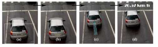
Inspired by the mentioned approaches for vehicle detection and speed measurement, in this article, we implemented a parallel version of the vehicle speed measurement approach presented in [12]. The main reason for choosing this method is its robust performance, containing computationally intensive modules and the high potential of parallelization according to the authors’ claims. This method takes advantage of license plate text features but does not require the characters of the license plate to be accurately segmented by the OCR algorithm to detect and track vehicles. Instead, the whole text appeared inside the license plate zone is recognized and tracked. The overall process of this approach includes four sequential steps, as it is shown briefly in Fig.2.

The first step is to find the moving objects – i.e. vehicles - among consecutive frames in order to limit the whole process to a set of regions. This goal was reached using MHI motion detection algorithm presented in [29]. Then, the moving parts of the scene were considered as vehicles’ boundaries and separated from the background scene. The frame differencing method produces a threshold binary image D(x, y, t) where the pixels with value 1 in each frame are segmented and other remained pixels, use the maximum value of the same rate in the previous frame. This collection of the output pixels is stored as H(x, y, t) in each frame which is shown in Equation (1), where τ refers to the duration of the motion in sequential frames.

Iт                if D ( x . "У . t )=1

max(0. H ( x . У . t -1)-1) о . w .

Then, a binary segmentation mask M(x, y, t) is acquired from H(x, y, t) to collect the moving parts, where the values of H larger than zero are presented as one in the mask. This process is presented in Equation (2):

M ( x . У . t )= {¹ ifH ⁽ x ^. У ^.1)>0 (2) 0 о .w.

Formerly, by applying Vertical Projection Profile (VPP) [30], the left and right borders of vehicles are detected (considering the vehicles moving from the bottom to the top of the screen). VPP counts the number of pixels existed in each column of the mask M(x, y, t) and stores the values in an array VP with a length equal to the number of the mask’s columns. After smoothing and normalizing VP, the exact range of pixels refers to the vehicle’s presence in each frame are recognized and cropped by applying Find-Hills [12] method. By detecting the regions inside the vehicle’s cropped area, the candidates of being the vehicle’s license plate are extracted. Thus, some parts of the moving vehicle with a rectangular shape and white background are selected using Edge Extraction and Filtering method [31]. Furthermore, a module to merge neighboring edges remained after filtering is defined in which only the edges with a pre-defined size and ratio are selected using connected components labeling [32]. Among multiple candidates, using T-HOG [27] text descriptor which has been introduced in Section 2.1, the region with the most probability of being the vehicle’s license plate will be extracted. The T-HOG descriptor will be used as an input for a Support Vector Machine (SVM) classifier and the output of the classifier shows whether the region belongs to a text or non-text area. In the next step and by detecting the license plate’s region, a set of unique features inside the region is chosen for tracking. This process is done by good features extraction. The good feature, in this case, is a high-intensity region with some black pixels inside the white region, representing a vehicle’s license plate. This feature is then tracked by the pyramid KLT tracking method introduced in Section 2.1 to provide the motion vector of the moving vehicle. In addition, a timer triggers as the vehicle enters the region of interest and stops as it leaves the region. Finally, each vector can represent the instantaneous speed of the vehicle at a specified time in pixels-per-frame metrics. Thus, a mapping function to convert it to the kilometers-per-hour unit is necessary to be applied. As it has been proved in the pinhole camera model, for a single view of the scene, the homograph matrix HM [33] can perform this mapping. Thus, according to the Equation (3), a plane-to-plane projective transformation and inverse perspective mapping can provide the final world plane metrics [37], where for a 3x3 homograph matrix HM, point p(xt,yt) can be mapped to the point p^(xw,yw) in the world plane [36]:

Г x_w -1 г zx_w -1            г ^x i -1

[ y_w ] = [ zy_w] = MM [ y]          (3)

HM can be obtained from four points in the image with known coordinates in the real-world plane in the calibration step. These features are utilized to present the relocation of the vehicle and calculate its speed by mapping pixels-to-meters and frames-to-seconds.

As it has been acknowledged in the paper, the process of calculating H(x, y, t) and M(x, y, t) matrices is computationally intensive. To solve this issue, the author suggested to apply subsampling function [12], but it still would be a bottleneck for the performance of the system. We will discuss the structure of parallelization for better performance in Section 3.

• III.    P roposed M ethod

For parallelization, some time-consuming modules of the mentioned method were detected and implemented on GPU using CUDA programming environment. Although the mentioned approach is robust against high accuracy performance, it is considered as a time-consuming method due to containing multiple computationally intensive modules. In this section, the implementation of a CUDA-enabled version of the same method is presented in order to decrease the time required for execution. To investigate the effects of each module in the performance, we implemented the same approach

• [12] . Fig.3 shows the time portion required for the execution of each module obtained by the means of profiling technique. To gather these time-shares, the implemented method was executed on several videos and the presented values are the average of the multiple calculated measures.

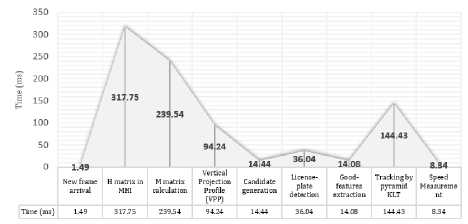
Fig.3. The time portion of various modules in the system (in milliseconds).

As it can be seen, the calculation of H(x, y, t) and M(x, y, t) matrices takes the most portion of time among the whole process, respectively. Vehicle tracking using the pyramid KLT is another computationally intensive module. In this regard, the system consumes totally 870.35 milliseconds to process the scene in order to detect and track vehicles in each frame; while the three mentioned modules consume 80.67% of the total time. The main reason of the huge time consumption in H(x, y, t) and M(x, y, t) matrices calculation is due to the system requirement for repeatedly performing the calculation for each pixel. These two modules have a rich data parallelism capability because they are made up of nested matrix multiplication operations. In addition, in the pyramid KLT tracking phase, the process of downsizing the vehicle’s image and drawing motion vectors in each level of the pyramid needs a huge amount of calculations. According to Fig.3, VPP is another computationally intensive module which does not support running across multiple cores in parallel.

To optimize the performance of these three timeconsuming modules, we want to perform a parallelization by implementing their CUDA-enabled versions. In the parallel implementations, data-parallel portions of each module should be implemented as a CUDA kernel, where these kernels are manipulated by the main processor, i.e. CPU. Consequently, a 30×30 matrix of pixels was allocated as a block to the GPU to optimize the calculating process. A block is a group of threads referring to each pixel that should be processed and by aggregating them into Grids , the architecture of a parallel version of each module will be shaped. The parallelization logic should distribute light calculation workloads (such as matrix multiplication) of the selected modules on each thread with the lowest data fetching overhead and optimal memory allocation.

Fig.4 shows the architecture of a GPU in brief [39]. According to Fig.4, there is a shared memory module and several registers inside each block which are allocated for calculations and shared for all threads of the block. In addition, each thread of a block has a unique local memory to store non-local variables, which are placed outside of the block. On the other hand, other memories including global, texture and constant memories are considered in GPU’s architecture for higher efficiency and better control of processes and shared by all threads inside the Gird. Consequently, to provide a high-efficiency system, it is necessary to utilize these memories and registers by the means of the CUDA platform.

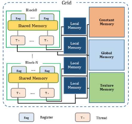
Fig.4. A common architecture of a GPU.

In order to parallelize H(x, y, t) , M(x, y, t) and pyramid KLT modules, we need to utilize GPU threads for each light-weight process. Fig.5 shows the CPU-based (sequential) version of MHI calculation according to Equation (1). As can be seen, all the pixels belong to the subtraction matrix of two sequential frames, named as diff should be checked as it was previously discussed in Equation (1). The current value of MHI module which is called H in this figure is the output of the system based on the previous frame’s MHI value prev . It should be noted that the variable mhi_duration is set to 5 in this approach, which means the system keeps tracking of five frames as the history to calculate the H matrix.

Algorithm!: Sequential H(x, y, t) Matrix Calculation input subtraction matrix diff of two sequential frames, previous frame’s H matrixprev, current frame’s H matrix H

• 1.    mhi duration C~ 5

• 2.    for all pixels p in rows of Jy/matrix do

• 3.      for all pixels p in columns of diff matrix do

• 4.        if^^T¹^] equals 1 then

• 5.             H [p] £■ mln duration

• 6.           else

• 7.            H [p] <- prev И - 1

• 8.          end if

• 9.    end for

• 10.    end for

output ZZ matrix

• Fig.5.    Sequential implementations of H(x, y, t) module.

In addition, Fig.6 shows the pseudo-code of the parallelized version of Algorithm1 presented in Fig.5. In this case, the block-size of the GPU is set to 30×30 which provides the best performance according to experiments and the resolution of the frames, named as w and h are utilized to calculate the grid based on block-size. In the parallel implementation, all the elements of the matrix diff are sequentially segmented into blocks and each block element should dedicate into a single processing thread. The pixels to thread mapping is done in O(1) and the row-major fetching of the diff matrix element, makes the H matrix calculation process to run in O(w+h) instead of O(wh).

Algorithm!: Parallel H(x, y, t) Matrix Calculation input subtraction matrix diff of two sequential frames, previous frame’s H matrixprev, current fr ame’s H matrix H, frame width w, frame height h

• 1.    define block [30] [30]

• 2.    define gird [W3 0] [Л/3 0]

• 3.    mhiduration 4- 5

• 4.    segment diff matrix to blocks and grids

• 5.    map each element in ti^matrix to a thread th

• 6.    for each element index in diff matrix do

• 7.    if й^[тг7ех] equals 1 then

• 8.    77[r»tifex] ^- mhi duration

• 9.       else

• 10.    Zf [zWex] 4- prev [Мех] - 1

• 11.      end if

• 12.    end for

output H matrix

• Fig.6.    Parallel implementations of H(x, y, t) module.

Similarly, Fig.7 and Fig.8 show the CPU-based (sequential) and GPU-based (parallel) versions of M(x, y, t) matrix calculation method. As it has been described before, M(x, y, t) matrix is used for segmentation of MHI . Here, variable M refers to the calculated mask M(x, y, t) presented in Equation (2). The parallelization process of this module was the same as the method described in Fig. 6.

Algorithms: Sequential M(x, y, t) Matrix Calculation input MHI matrix H

• 1.    for all elements p in rows of H matrix do

• 2.    for all elements p in columns of H matrix do

• 3.         ifZ/[p] >  0 then

• 4.             Af|>] 4- 1

• 5.           else

• 6.             Л/[р] 4- 0

• 7.          end if

• 8.    end for

• 9.    end for

output M matrix

Fig.7. Sequential implementations of M(x, y, t) module.

Algorithm4: Parallel M(x, y, t) Matrix Calculation input MHI matrix H, frame width w, frame height h

• 1.    define block [3 0] [3 0]

• 2.    define gird [w/3 0] [Л/3 0]

• 3.  segment H matrix to blocks and grids

• 4.    map each element in //matrix to a tluead th

• 5.    for each element index in H matrix do

• 6.       if H [imt/ex] > 0 then

• 7.        M [Wex] 4- I

• 8.        else

• 9.       JW[Wex] 4- 0

• 10.      end if

IL end for output Af matrix

Fig.8. Parallel implementations of M(x, y, t) module.

In addition, Fig.9 shows the output of the produced mask in the motion detection step. As it is shown, the moving vehicle in multiple frames is totally segmented from the background scene.

Finally, Fig.10 and Fig.11 illustrate the sequential and parallel versions of the pyramid KLT module, respectively. In these figures, previous and current frame matrices with the resolution of w × h are utilized to detect any relocation of the objects with special visual features and provide tracking of them in two sequential frames. These matrices are named prev_frame and curr_frame and the candidate features of being a license plate found by the good features algorithm are stored in prev_features and the curr_features arrays, respectively.

Firstly, the algorithm builds a pyramid with multiple levels, where the variable max_level defines the number of levels.

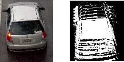
(a)                                    (b)

Fig.9. A sample frame (a), its binary segmentation mask M (b).

Algorithms: Sequential Pyramid KLT Method _____________________________________ input previous, frame’s matrix preV-framefw][h], current frame’s matrix curr'-framefw][h], previous frame's features preV—features, current frame's features curr-features, output status vector status, output vector of errors err, maximum number of iterations tc

• 1.    tc <■ 30

• 2.    max level fr 5

• 3.    for index i = 0 to max_level do

• 4.     pyramid_prev_/rame[i][H’/i+l][M+J] ^* 0

• 5.      pyramid curr /rame[i][w/i+l3[li/i+Jl 4~ 0

• 6.      scale e (i + 1)*2                   "

• 7.    for index/ = 0 to wdcale do

• 8.        for index к = 0 to h/scale do

• 9.             pyramid_preV-framef] И[Аг] ^r prev_frame\i*scale]\k*scale]

• 10.           pyramidcurr _/ratne[i] [/][£] 4- curr_framef*scale\\k*scale\

• 11.    end for

• 12.    end for

• 13.    end for

• 14.    for each pyramid level i in.pyramid_curr_frame do

• 15.     derjr. fr derivative ofpyramidcurrjrame with respect to x

• 16.     derpy f~ derivative ofpyrtzmidcurr-frame with respect to у

• 17.    Create spatial gradient matrix G from derx and derpy

• 18.    for counter = 0 to tc do

• 19.       if feature E ^prev-features & curr-features } then

• 20.            stains feature] 4- 1

• 21.       else if feature 6 { preV-features & curr-features } then

• 22.             status feature] fr 0

• 23.    else

• 24.             err feature] fr 0|

• 25.       end if

• 26.    Create image mismatch vector № for this level from status and err

• 21.       OpticalFlow = G'Pksv

• 28.    end for

• 29.    end for

output final OpticalFlcm vector for all pyramid levels

• Fig.10.    Sequential implementations of the pyramid KLT tracking module.

Each detected license plate from the detection step of the method lays in the base level of the pyramid and each higher level, stores the image of the license plate with half dimensions. Each pyramid version of the prev_frame and curr_frame frames are stored at pyramid_prev_frame[i] and pyramid_curr_frame[i] respectively, where i is the corresponding level of the pyramid. After building the pyramid, if a feature found in both previous and current frames, its corresponding element in the status array becomes one and otherwise, it becomes zero. Similarly, the array err includes the type of errors occurred in tracking the corresponding feature. In addition, the variable tc stores the terminating conditions of the search module and the maximum number of pyramid levels is set to five by experiment in this approach. Finally, the OpticalFlow variable includes the required features for tracking the license plate in later frames. It should be noted that in the proposed implementation, we considered 10 frames for tracking, instead of tracking the vehicle in the whole scene and no huge changes in tracking accuracy were detected. Fig 11 indicates the parallel implementation of Algorithm5 in a CUDA-enabled environment. According to [40], the parallelized version of the KLT tracking algorithm can provide a large rate of speed-up due to containing multiple add, subtraction, and multiplication matrix processes. The definition of block and grid is the same as Algorithm2 and Algorithm4. The pixels to threads mapping is done in O(1) and the row-major fetching of the pixels in each pyramid level is executed in parallel. It should be noted that the implementation codes of both CUP-based and CUDA-enabled version of Algorithms1 to 5 are presented in the Appendices section.

AlgorithmS: Parallel Py ramid KLT Method ______________________________________________ input previous frame’s matrix prevJrame[xv] [h], current frame’s matrix currJrame[xv] [h], previous frame’s features prev Jeatures.. current frame’s features curr Jeatures, output status vector status, output vector of errors err, maximum number of iterations tc

• 1.    tc ^r 30

• 2.    maxlexel ^- 5

• 3.    define block [30][30]

• 4.    define grid [w/30] [й/3 0]

• 5.    for index i = 0 to mox_/eveZ allocated to threads do

• 6.     pyramid_prevJrame[i][xv/i+7][h/i-H] ^~ 0

• 7.     pyramid_currJrame[i][xv/i+7][h/i+7] ^* 0

• 8.     segment pyramid_prevJrame and pyramid_currJrame matrices to blocks and grids

• 9.    map each element pyramid_prevJrame and pyramid_currJrame to a thread th

• 10.    for each thread r/? dedicated to block elements do

• 11.       size of pyramid_prevjrame level z+1 ^ (prevjrame size level z) / 2

• 12.       size of pyramid_currJrame level z+1 ^~ (currJrame size level i) / 2

• 13.    end for

• 14.    end for

• 15.    for each pyramid level i in pyramid_currJrame do

• 16.    calculate der_x and der_y by thread

• 17.    Create spatial gradient matrix G from der_x and cfer_j'

• 18.    for counter = 0 to tc allocated to threads do

• 19.        i$feature E (prevJeatures & curr Jeatures } then

• 20.             status [feature] ^~ 1

• 21.       else if feature £ { prex Jeatures & curr Jeatures } then|

• 22.             status [feature] ^- 0

• 23.    else

• 24.             err [feature] fr 0

• 25.       end if

• 26.    Create image mismatch vector mv for this level from status and err

• 27.       OpticalFlow = (jfmv

• 28.    end for

• 29.    end for

output final OpticalFiow vector for all pyramid levels

• Fig.11.    Parallel implementations of the pyramid KLT tracking module.

  

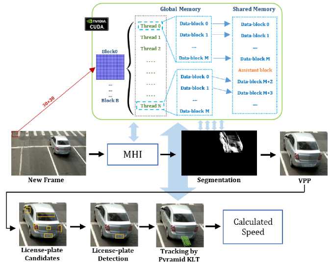
  Fig.12. The overall diagram of the proposed parallelized speed measurement system.

  
  

As a summary, Fig.12 demonstrates the overall process of the speed measurement approach and the proposed parallelized modules. As it can be seen, we have considered a 30×30 block of pixels for parallelization of MHI and segmentation modules, i.e. calculation of H(x, y, t) , M(x, y, t) matrices, respectively. On the other hand, the parallelization of the pyramid KLT was done in each level of the pyramid to track the vehicles in sequential frames. Consequently, each block contains N+1 threads and each thread works on M+1 data blocks on the global memory. The final results of the processes are transferred to the shared memory.

• IV.    E xperimental R esults

This section introduces the performances of the parallel implemented method presented in this article in terms of time execution. Both the parallel (GPU-enabled) and sequential (proposed in [12]) methods were analyzed on a computer with properties demonstrated in Table 1. We describe the experiment by introducing the main factors utilized for time consumption comparison.

• A.    Dataset

The provided dataset for the experiment is a video dataset which has been captured via a camera installed above an urban roadway. The dataset is provided by the Federal University of Technology of Paraná (FUTP) [12], including five H264 videos captured by a 5-megapixel CMOS image sensor with different illumination and weather conditions summarized in Table 2. The video has been captured the rear view of vehicles, makes it suitable for license plate detection and speed measurement purposes. It has to be mentioned that due to different types of motorcycles’ license plates, they have been skipped in this paper [12]. Frame resolution of the dataset is 1920×1080 pixels and the frame-rate is 30.15 frames per second. The videos are categorized into five different categories according to weather and recording conditions. Each video has a separate XML file format that contains information about that video such as vehicle speed. Table 2 shows the properties of this dataset with its corresponding speed ranges.

Table 1. Implementation Hardware And Environment
Hardware	Properties
CPU	3.5 GHz Intel Core i7 – 7500U
RAM	12 GB
GPU	NVIDIA GEFORCE 920MX
Operating System	64-bit Windows 10

Table 2. Properties Of The Dataset.

Dataset	Filename	#frame	Video properties	#Vehicles
The Federal University of Technology of Paraná [12]	Set01_video01	6918	Normal illumination	119
	Set02_ video01	12053	High illumination	223
	Set03_ video01	24301	Low-light illumination	460
	Set04_ video01	19744	Rainy weather conditions	349
	Set05_ video01	36254	Extreme rain weather	869
Total	-	99270	-	2020

• B.    Time Consumption

To evaluate the performance of the parallelized method, we have compared it to the sequential method presented in [12]. Since there were no vast changes in the accuracy of vehicle detection, tracking and speed measurement processes in the parallelized and sequential approaches, we have only focused on the timeconsumption comparison. By comparing elapsed times for execution of the parallelized versions of H , M and Pyramid KLT modules to the original, we observed a huge change in the fields of performance and efficiency. Table 3 shows the results of this evaluation in brief. It should be noted that each cell of the table refers to the average elapsed time for a particular vehicle to run the mentioned modules in different videos. As it can be seen, the parallelized versions (kernels) execute 188.87, 408.71 and 21.28 times faster than the sequential versions in calculating H , M and Pyramid KLT modules, respectively.

According to Table 3, only the effect of parallelization on each module H, M and Pyramid KLT are presented in terms of speed-up. In other words, Table 3 only shows the effect of parallelization on each kernel, while the whole effect of utilizing these modules in the application level is not provided. In order to review the effects of parallelization on the whole process of speed measurement, Fig.13 illustrates the average of the total time required to calculate a single vehicles’ speed in various videos of the dataset. As can be seen, parallelization of the most computationally intensive modules leads to about 1.81 execution speed-up in application level in various illumination and weather conditions. To acquire these numbers, a timer triggered as a vehicle entered the ROI with a recognizable license plate and stopped as it left the region. Although the parallelized versions of H, M, and Pyramid KLT modules provide a robust speed-up according to Table 3, the effect of utilizing them in the speed measurement process did not provide a vast difference, as it can be seen in Fig.13. The reason can be found in the huge amount of data transportation among GPU and CPU for processing.

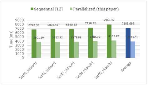
Fig.13. Total running time of sequential and CUDA-enabled implementations to calculate the speed of a single vehicle on various videos.

Table 3. Time Consumptions Of Sequential And Parallelized Implementations Of Modules For Each Vehicle.

Dataset	Filename	H(x, y, t)		M(x, y, t)		Pyramid KLT
The Federal University of Technology of Paraná [12]	Set01_video01	CPU	GPU	CPU	GPU	CPU	GPU
	Set02_ video01	318.93	1.54	272.76	0.18	132.71	6.02
	Set03_ video01	285.42	1.33	224.85	0.43	144.56	6.49
	Set04_ video01	341.72	2.19	242.12	0.82	150.25	7.73
	Set05_ video01	315.07	1.68	218.74	0.68	146.23	6.89
Average		321.64	1.64	247.22	0.84	151.42	6.94
Speed-up		316.56	1.68	241.14	0.59	145.03	6.81
		188.87		408.71		21.28

Finally, to provide a better demonstration of the parallelization effect on each distinct modules of the proposed speed measurement approach, Fig.14 presents the time portion required for the execution of each essential module in brief. As it can be seen, the chart shows the execution time (in milliseconds) of each distinct modules of the parallelized version in comparison with the sequential version, which has been previously presented in Fig.3. It should be noted that to acquire these execution times, the time wasted to transfer data between GPU memories and CPU are skipped. On the other hand, the effect of parallelization on the accuracy of the system compared to the sequential version was negligible.

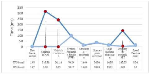
Fig.14. Profiling time portion of various modules in the system (in milliseconds).

According to Fig.14, the huge gap between H, M and Pyramid KLT modules are obviously distinct (shown in red dots for both sequential and parallelized versions). As a result, the benefits and advantages presented in the experiments are adequate to make the CUDA-enabled version more applicable in almost real-time applications.

• V.    C onclusions

Intelligent Transportation Systems are used in various traffic-related applications such as roadway monitoring and vehicle counting. By utilizing cameras in ITS applications, Video-based Intelligent Transportation Systems were appeared, which can be used in various applications like speed measurement. In this paper, a parallelized version of a formerly-proposed vehicle speed measurement method is presented which has the advantage of appropriate time consumption, accuracy, and robustness. The CPU-based version of the mentioned method has three modules including vehicle detection, tracking, and speed measurement. We have realized that two functions in vehicle detection and one in the tracking phase are computationally intensive and have the potential to be highly reduced in cost. By implementing the same method in a CUDA-enabled environment and applying data-level parallelism on these modules, better throughputs and performance have been obtained. Experimental results showed that the parallelized version of the method provides 1.81 speed-up in application level to measure each vehicle’s speed compared to the normal CPU-based implementation in overall. In addition, the kernel-level parallelization provided 21.28, 408.71 and 188.87 speed-up in executing three computationally intensive modules.

A ppendices

Appendix I - Sequential and parallel implementations of H(X, Y, T) module in C++

Below, the variable diff_mat refers to the subtraction matrix of two sequential frames. If the result of the subtraction was equal to 1, the first condition of Equation (1) is used and otherwise, the second condition would be utilized. In addition, variable current_mhi refers to the current value of MHI and prev_mhi represents its value in the previous frame. The variable mhi_duration is set to 5 in this approach, which means the system takes advantage of five frames as the history to calculate the H matrix. In the CUDA-enabled codes, the block-size of the GPU is defined in BX and BY and the resolution of the frames are defined in DX and DY, respectively. In addition, the function type qualifier __global__ refers to a kernel with the ability to be executed on the CUDA device and grid and block variables, contain the dimensions of grids and blocks. The block size is set to 30×30, which provides the best performance according to experiments. In addition, _Update_MHI_GPU is the name of kernel and row and col variables are used to choose threads. The provided pseudo-codes of these two implementations are shown in below.

CPU:

}

GPU (CUDA):

#define BX 30    #define BY30

#define DX 1920  #define DY1080

dim3 block ( BX , BY );

dim3 grid ( DX / block . x , DY / block . y );

DY , DX , mhi_duration );

Function :

__global__ void  _Update_MHI_GPU(uchar*  current_mhi, uchar* prev_mhi,  uchar*  diff_mat, size_t step, int h, int w, int mhi_duration) { int row = blockIdx.y * blockDim.y + threadIdx.y;

int col = blockIdx . x * blockDim . x + threadIdx . x ;

int index = col + row *( step / sizeof( uchar )); if ( index >= ( h * w ))

return;

if ( diff_mat[index] ==)

current_mhi [ index ] = mhi_duration ;

else if (prev_mhi[index] >)

current_mhi[index] = prev_mhi[index] -;

}               ""

Appendix II - Sequential and parallel implementations of M(X, Y, T) module in C++

Below, the CPU-based (sequential) and GPU-based (parallel) implementations of M(x, y, t) matrix calculation method are shown, where _SegmentationBy_GPU is the name of the kernel. As it has been described before, M(x, y, t) matrix is used for segmentation of MHI . Variable m_mat refers to M(x, y, t) matrix presented in Equation (2), thus if the value of MHI was bigger than zero, the value of M would be 1 and otherwise, it stores as zero. Pseudocodes of these two implementations are shown in below.

CPU:

}“

GPU (CUDA):

#define BX 30   #define BY30

#define DX 1920 #define DY1080

dim3 block ( BX , BY );

dim3 grid ( DX / block . x , DY / block . y );

Function :

__global__ void _SegmentationBy_GPU(uchar* m_mat, uchar* mhi, size_t step, int height, int width) { int row = blockIdx.y * blockDim.y + threadIdx.y;

int col = blockIdx . x * blockDim . x + threadIdx . x ;

int index = col + row *( step / sizeof( uchar ));

if ( index >= ( height * width )) return;

if (mhi[index]> m_mat[index] =;

else m_mat[index]=

}"

Appendix III - Sequential and parallel implementations of the pyramid KLT tracking module in C++

Below codes illustrate the sequential and parallel implementations of the pyramid KLT module. According to these codes, prev_frame and curr_frame variables refer to the current and previous frames matrices, respectively. The candidate features of being a license plate found in the previous frame by the good features algorithm are stored in prev_features and the curr_features variable keeps the features existed in the current frame. Finally, variable tc stores the terminating conditions of the search module. Pseudocodes of these two implementations are shown in below.

CPU:

TermCriteria tc = TermCriteria ( TermCriteria :: COUNT + TermCriteria :: EPS , 30 , 0.01 );

CalcOpticalFlowPyrLK   (prev_frame, curr_frame,  prev_features, curr_features, status, Size (   ,    ), 5, tc, 0 , 0.0001);

GPU (CUDA):

Ptr<:sparsepyrlkopticalflow> d_pyrLK_sparse = cuda::SparsePyrLKOpticalFlow::create(Size(11, 11), 5, 1);

d_pyrLK_sparse -> calc ( prev_frame , curr frame ,    Prev Points ,

Next_Points , d_status );