Passivity analysis of neutral fuzzy system with linear fractional uncertainty

Published Online March 2011 in MECS

The Takagi-Sugeno (T-S) model [1] has been paid considerable attention in the past two decades. It has been shown that the T-S model method gives an effective way to represent complex nonlinear systems by some simple local linear dynamic systems, and some analysis methods in the linear systems can be effectively extended to the T-S fuzzy systems. Recently the T-S fuzzy neutral system has been introduced in [2] and the stability and stabilization analysis of fuzzy neutral systems have been extensively investigated, see, e.g.,[2-6] and the references therein.

On the other hand, The delay varying in an interval has strong application background, which commonly exists in many practical systems. For example, it has been described in [7] that the lower bound of the delay in the networked control systems is often larger than zero. The investigation for the systems with interval time-varying delay has been caused considerable attention, see [8-11] and the references therein.

The passivity theory, intimately related to circuit analysis methods, has received a lot of attention from the control community during the last several decades, see, e.g., [12,13]. It provides a nice tool for analyzing the stability of systems, and has found applications in diverse areas such as stability, complexity, signal processing. The fuzzy control systems associated with passivity have been studied preliminarily in [14]; [15] investigated the passivity and pacification of uncertain fuzzy systems; By utilizing the Lyapunov functional method, the Itoˆ differential rule and the matrix analysis techniques, the passivity and pacification problems have been investigated for a class of uncertain stochastic fuzzy systems with time-varying delays [16].

However, to the best of the authors’ knowledge, the passivity analysis of T-S fuzzy neutral system with interval time-varying delay and linear fractional parametric uncertainty has not been addressed, which motivates the present study.

Notations. R" and Rnxm denote, respectively, the n-dimensional Euclidean space and the set of all n x m real matrices. The notation A > B means that A — B is ur positive definite. A represents the sum of A and its transpose. I is the identity matrix with appropriate dimension. “*” denotes the elements below the main diagonal of a symmetric block matrix. L2 [10, да) denotes the space of square integral functions on [10, да) .

Project supported by the Scientific Research Fund for “PhD Talents Introduction” of CAFUC (No. J2009-40).

• II.    PROBLEM FORMULATION

In this section, a class of neutral T-S fuzzy systems with interval time-varying delay and linear fractional parametric uncertainty is considered. For each i G S=@ {1,2,L , r }, where r is the number of plant rules, the i th rule of T-S fuzzy model is represented as follows:

Plant Rule i: IF z. (t) is M.., z_ (t) is Mn ,L , z (t) 1                i1      2                i2             p is M , THEN ip

' x( t ) = A ( t ) x ( t ) + B , ( t ) x ( t - t( t )) + C , ( t ) X( t - t( t ))

,        + D,w (t), y (t) = Ex (t) + Fx (t - t( t)) + H w (t),

_x(t) = ^(t), t £[-TM,0], where z1 (t), z2 (t), L , zp (t) are the premise variables, and each M,1(1 = 1, 2, L , p) is a fuzzy set; x(t) £ R" is the state variable, y(t) £ Rm is the output vector, w(t) £ R1 is the disturbance input belonged to L2 [10, да) ; ^(t) : [-TM, 0) ^ R" is a smooth vector-value initial function;

t ( t ) g [ T m , T M ] is the interval time-varying delay, where

0 < T < T,, and T(t) < d ; D , E., F, H are constant m M                             ,    ,    , matrices with appropriate dimensions; A (t), B (t),

C ( t ) are matrices with appropriate dimension and admissible linear fractional parametric uncertainties, that is, these matrices satisfy

[A (t), B (t),C (t)]

= [ A , B , , C , ] + L A (t ) [ E_u, E 2 , , E 3 , ],

A(t) = [I - F(t) JГ1 F(t),

I - JJ > 0, where A, B, , C,, L,, E, (1 = 1,2,3) and J are known real constant matrices with appropriate dimension, and F(t) is a matrix function satisfying

F (t) FT (t) < I.

Remark 1. The uncertainty A ( t ) satisfying (3)-(5) is referred to as a linear fractional parametric uncertainty. Note that when J = 0 , A ( t ) reduces to a norm-bounded parametric uncertainty that has been extensively investigated in the study of robust control problems.

Applying a center-average defuzzier, product inference and singleton fuzzifier, the dynamic fuzzy model in (1) can be represented by

К t ) = E A ^{( z (} t ^))[ A ⁽ t ) ^{x (} t ) ^{+ B} , ⁽ t ) ^{x (} t ^{- t (} t ))

+ C ( t ) & t - t ( t )) + Dw ( t )],

У ⁽ t ) = E A ^{( z (} t ^))[ Ex ⁽ t ) ⁺ F^{x (} t ^{- t (} t)) ^{+ H}w ⁽ t )1,

=1

_ x ( t ) = y (t ), t g[- T m ,0],

(6) where

A ( z ( t )) = .    £1 M l ( z i ( • ))

E„ , n p ., M ,1 ( Z i ( t ))

with z(t) = (z1(t), z2(t),L ,Zp(t)); M,1 (Zi(t))is the grade of membership of zl (t) in M l ; For notational simplicity, A, is used to represent A,(z(t)) in this paper. By the definition in (7), it follows that A, — 0 and E r., A, = 1.

Definition 1 [17]. The system (1) is called passive if there exists a scalar у >  0 such that tt

• ^-Y J 0 ^{w (} s ) ^{w (} s ) ^ds <  ² J ₀ w^{T (} s ) У ^{( s} ) ^ds , t p ^{— 0}

for all solution of (1) under zero initial condition.

Lemma 1 [18]. Suppose A ( t ) is given by (3). Given matrices M = M ^T , L and E of appropriate dimension, the following statements are equivalent:

• (i)    the inequality

M + L A ( t ) E + E^T A ^T ( t ) L T <  0

holds for all F ( t ) satisfying F ( t ) F^T ( t ) <  I ;

• (ii)    for 8 >  0

  Г M	8 ET	L "
  *	- 8 I	8 JT	< 0.
  *	*	- 8 I _

Lemma 2 [11]. Let E 1 , E ₂ and Q be constant matrices appropriate dimensions and 0 <  T m <  t ( t ) <  T _M , then ( ^T ( t ) ^{- T} m ^{) E} 1 ^{+ ( T} M - ^T ( t ^{)) E} 2 ^{+ Q}<  ⁰ if and only if

(TM - Tm )E1 +Q< 0

and

(TM - Tm )E2 +Q< 0

hold.

III. MAIN RESULTS

Theorem 1 . For a prescribed у >  0 , scalars T m and T M , the system (1) is passive if there exist scalars s i ( i £ S ) , matrices P >  0, Z >  0, Q, ( l = 1,2,3), S, >  0, S, >  0, l      kk

M ki , N_ki , ( k = 1,2; i £ S ) such that the following LMIs hold

■qi      Лi      S1 3(l) siET Li ■ uu* * -yI - Hi    0     0     0 Si(l) = *      *      - R 2    0     0 < 0, *       *        *     -£iI £iJT _ *        *         *       *     -£iI _ l = 1,2; i £ S

where	3 - R 1 + 2 Q l l = 1 *	p + a t s T Q 22	R 1 0	0 Q 24
Q i =	*	*	Q 33	Q 34
	*	*	*	Q 44
	*	*	*	*
	.      *	*	*	*

0	A T S T     "
0	S 1 C i - S T
0	0
T N 2 i   N 1 i	B f s T
uur
- Q 3 - N 2 i	0
	uuuur
*	-(1 - d ) Z + S 2 C i

Л f = [ - E i , D T S f ,0, - F i ,0, D T S T ],

S i ³(1) = V T m - T m M i , S ³(2) = V T m -T m N ,

E i = [ E .,0,0, E ₂Л E 3 i ],

L■ = [0, LfSf ,0,0,0, LfS2T ], wt MT = [0,0, Mf, M T,0,0],

N T = [0,0,0, N T , N T ,0],

Q22 =-S + Ы + (Tm - Tm )R2 + Z],

Q 24 = S 1 B i ,

ULU

Q 33 =- Q_x - R + M _lp Q 34 = MT- M _u, uur uuur

Q 44 = - (1 - d ) Q 2 + N _u- M 2 i .

Proof. Choose the Lyapunov-Krasovskii functional as follows:

V ( x t ) = V ( x t ) + V 2 (x_t ) + V 3 ( x t ) + V 4 (x_t ),    (9)

where

V:( x) = Г t -T

m

V(xt) = xT (t) Px (t), xT (5) Q1 x (5) ds + [    xT (s) Q2 x (s) ds

J t -T ( t )

+ f    x^T ( s ) Q ₃ x ( s ) ds ,

^1-TM

V( x t ) = T m f f f ( e ) R f ( e ) d e ds

^-T „ sS

+ [ ' ' " rT^r ( e ) r f ( e ) d e ds , J t -T m ss

V 4 ( x_t ) = Г ₍f T ( s ) Z f s ) ds Jt -t ( t ) with f t ) = x ( t ).

Taking derivative of V ( x_t ) along the trajectory of the system (6), we have

Vx_t ) = V ( x_t ) + V 2 ( x_t ) + V 3 ( x_t ) + V 4 ( x_t ),    (10)

where

V ( x_t ) = 2 x^T ( t ) P f t ),               (11)

V 2 ⁽ x t ) = x T ⁽ t )( £ ³ = 1 ^Ql ) x ⁽¹) - x T ⁽¹ - ^T m ) ^Q 1 x ⁽¹ - ^T m ) - (1 - T &( t )) x^T ( t - t ( t )) Q ₂ x ( t - t ( t )) - ^xT ⁽ t ^{- T} M ) ^Q 3 ^{x (} t ^{- T} M )

^ x^{T (} t ⁾⁽ E ³ = 1 ^Ql ) x ⁽ t ) ^- x^{T (} t ^{- T} m ) ^Q 1 x ⁽ t ^{- T} m ) - (1 - d ) x^T ( t - t ( t )) Q ₂ x ( t - t ( t ))

• ^{-    x}T ⁽ t ^{- T} M ) ^Q 3 ^{x (} t ^{- T} M ),

V & ( x t ) = # ^T ( t )[ T „ R , + ( T m - T m ) R 2 ] f ( t )

• - T m f   f ( s ) R i ^ ( s ) ds

t ^-T m

• - f t - ^{T m} f ( s ) R 2 f ( s ) ds , t ^-T M

• V & ( x_t ) <  f ( t ) Z f ( t ) - (1 - d ) f ( t - t ( t )) Z f ( t - t ( t )).

(14) Employing the free-weighing matrix method [19-21], we have

• 2 2 P i ^ ⁽ t ) ^Mi ^[ x ⁽ t ^{- T} m ) ^- x ⁽ t ^{- T (} t )) ^- f ^T m a ^{f (} s ) ^{ds ]} = ⁰, ■^7                                                         ^J t^{-T (} t )

i = 1

2 2 mM ( t ) N[ [ x ( t - t ( t )) - x ( t - T m ) - J t ^{T (} t) e s ) ds ] = 0, i = 1                                                           t ^{- T} M

2 2 / = i m , M ⁽ t ) ^S i ^e t ) ⁺ A i ⁽ t ) x ⁽ t ) ⁺ B i ⁽ t ) x ⁽ t ^{- t(} t ))

+ C i ( t) x( t - t ( t )) + Dw ( t )] = 0,

(17) where

- ' ' ⁽ t ) = ^[ x T ⁽ t ), J T ⁽ t ), x T ⁽ t ^- m ) ), x T ⁽ t ^{- t (} t )), x T ⁽ t ^{- T} m ), M ( t - t ( t ))] and S T = [0, S T , 0,0,0, S T ] .

Then it follows from (10)-(17) that

V x,) - 2 wT (t) y (t) - yW (t) w (t)

< 2 xT (t) P£( t) + xT (t )(2 3=1 Q) x (t)

- xT (t - Tm ) Q1 x(t - Tm )

- (1 - d) xT (t - t( t)) Q2 x (t - t( t))

- xT (t - TM ) Q3 x(t - MM )

+ e (t)[TmRi + (Tm - Tm )R2 + Z]^(t)

• - mT e ( s ) R 1 ^ ( s ) ds ^j t- ^T „

• -Ц e (s) Re( s) ds

- (1 - d e (t - т (t)) ze t - t (t))

+ 22 Ы mP (t M [x(t - Tm ) - x(t - T(I))

- Г "T- e s ) ds ]

J t-T ( t )

+22 r=1 ^i^(t) N[ x(t- T (t))- x(t- tm )

f t -t ( t )

e(s) ds ]

^ t^-T M

+22 '=, Mt^ (t )s [-e( t)+At (t) x (t)

+ Bt (t) x (t - T (t))

+ Ct( t) ;8( t - T (t)) + Dtw (t)]

- 2 wT (t) y (t) - /wT (t) w(t).

Using Lemma 1 in [10], we have

-T _mV e ( s ) R_x e ( s ) ds ^j t ^-T m

<

T x (t)      -R1

. x ( t - T _m ) J L R 1

R 1

-

R 1

x ( t )

^{x (} t ^{- T} m )

Via the method in [7], we obtain

E V       rr        f t T'

,.1 M6 ⁽ 1 ) ^M, J , _ , ( t ) ^{e (} s ) ds

< f^{- T} - e ( s ) r, e ( s ) ds t - t ( t )

+ (T(t) - Tm )2/=1 Mi^ (t)MiR2 1 Mi- (t), and

-22 r-1 Mt^(t)Nt ГT(t)e(s)ds 1                it-TM ft-T (t)   _ e (s) R 2^( s) ds t-TM

+ ( T „ - t ( t )) 2 , '., «< ^T ( t ) NR 2¹ N T < ( t ).

So it follows from (18)-(21) that

V ( x, ) - 2 w^T ( t ) y ( t ) - Y W T ( t ) w ( t )

< 2 Г .1 M , ; ( t )[( t ( t ) - T m ) M , R 2¹ M , ^T

+ ( T m - т ( t )) N , R , ¹ N T +n , (t )] _f ( t )

+ 2 2 '„ M , ^ ( t )SDW ( t )

- 2 w^T ( t ) y ( t ) - Y w T ( t ) w ( t )

? ⁽ t )

Y , ( t )

Л , ur -Y I - H _t

= 2L Mi

^{1 1}      _ w ( t )

*

,(t)

W ( t ) J

(22) where

Y , ( t ) = ( T ( t ) - T m ) M , R 2 ^{- 1} M T + ( T m - T ( t )) N , R 2 ^{- 1} N T + Q , ( t ) and Q , ( t ) is obtained form Q , by replacing the terms

A , B , C with A ( t ), B ( t ), C ( t ) , respectively.

By the Schur complements, Lemma 1 and Lemma 2, the LMIs (8) give that

Y , ( t )

*

Л , ur

-YI - Н,

< 0, i■ G S. .

Then, it follows from (22) and (23) that

V ( x_t ) - 2 w^T ( t ) y ( t ) - Y w T ( t ) w ( t ) <  0-      (24)

Integrating (24) with respect to t over time interval [0, t p ], t p >  0, we have

V ⁽ x ) ^- V ⁽ x ₀) ^{- Y} t w^{T (} s ) w ⁽ s ) ds p                   J0

• < ² J ₀ ^P w ^{( s} ) y ^{( s} ) ^ds •

So, under the zero initial condition, we have

• - Y J ₀ t ^p w^{T ( s} ) ^{w ( s} ) ^ds <  ² J ₀ t ^P w^{T ( s} ) y ^{( s} ) ^ds •

The proof is completed here.

Remark 2. Letting J = 0 in (8) yields the Theorem 1 in [22]. In view of this, our results in the article extend the corresponding results in [22].

output. And the curve of

• IV.    SIMULATION EXAMPLE

In this section, a simulation example is given to illustrate the effectiveness of the developed approach. Consider the system (1) with parameters as follows

J ( t p ) =

-2\0 wT(5)у (5) ds J^ WT ( 5 )w ( 5 ) ds tP > 0

is provided in Fig. 3.

A -.	- 4 1.2	0 " - 5	,		" 2 = .	-3 0	06 1 -4
5 1 =.	1 0.5	0.4 1.3	,		В 2 = _	14 0.4	0.6 " 0.8_	,
C 1 =.	0.4 0	0 " - 0.2 _		,	C 2 =.	-0 .2 0	0 03		f
D 1 -	1.2 0.6	- 0.4 " 1.5 _		,	D 2 =	- 0.9 0.3	- 0.8 " 1 _		'
E 1 =	- 1.6 - 0.2	0.8 " 1.3 _		,	E 2 ="	-14 0.6	-0 .2 " 1.5 _		,
F =[	0.8 - 0.5	0.6 " - 1		,	F 2 =	"-1 _ 0	0.3 " 0.6_	,
H 1 =	"- 0.6 _ 0.4	-	0.5 1	"	, H 2 =	" 12 _ 0.4	0.6 " - 0.5 _		,
L 1 =	" 1 _ 0.6	- 0.4 " 1.2 _		,	L 2 =	"0 6 _0 2	0 0 .8	"
E 11 =	" 0.6 _ 0.2	- 0.3 " 0.7 _		,	E 12 =	" 1.2 _ 0.4	0 " - 0.5 _		'
E 21 =	- 0.8 0.5 -		0 " -1.2 _		E 22 =	[ —I _ 0	0 .3 0 .4	5	,
E 31 =	1.2 0	- 0.6 - 1			E 32 =	"0 8 _0 4	02" -*H_		,
J =	" 0.2 0	0 " 0.1		,	F ( t ) =	sin t 0	0 cos t

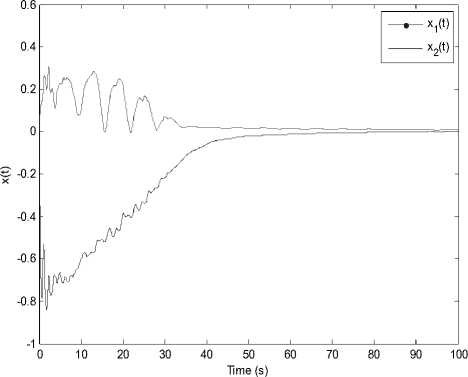
Fig. 1. State response x ( t ).

т ( t ) = 1 - 2sin t .

Choose the scalar / = 1.25 , then solving the LMIs in (8) via the algorithm “ feasp ” in Matlab, it is found that these LMIs are feasible. So, according to Theorem 1, the system (1) is passive. For convenience of the simulation, let

Ц 1 ( t ) = sin(^ 1 ( t )), ц ₂ ( t ) = 1 - sin(^ 1 ( t )) and

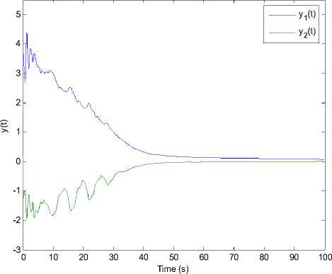
Fig. 2. System output y ( t ).

w ⁽ t ) =

1 + t

1     " T

2 + 0.3 t

, t >  0.

Then, the simulation results of the state response of the plant is given in Fig.1, while Fig.2 shows the system

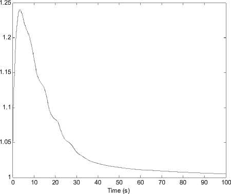
Fig. 3. The curve of J ( _{t ρ} ) .

• V.    CONCLUSION

This paper has investigated the passivity problem for the T-S fuzzy neutral system with interval time-varying delay and linear fractional parametric uncertainties. Delay dependent sufficient conditions for solvability of the passive problem are obtained by means of the Lyapunov-Krasovskii functional and the free weighting matrix method. The presented criterion in terms of LMIs can be readily solved via the standard numerical algorithm in Matlab. Finally, a simulation example is provided to demonstrate effectiveness and applicability of the theoretical results.

A CKNOWLEDGMENT

The authors would like to thank ICIECS2010 and the anonymous reviewers for their helpful and insightful comments for further improving the quality of this work.