Pattern Formation in Swarming Spacecrafts using Tersoff-Brenner Potential Field

Published Online May 2013 in MECS

With the development of MEMS (Microelectromechanical Systems) technology [1], people pay more attention to micro spacecraft, which makes an excellent complement to large spacecraft. Especially, micro spacecrafts can be swarmed by a suited control law to form a virtual large spacecraft, that is, the swarming ones can not only realize the function of large one, but also may exceed it, since swarming system has the following advantages:

• 1)    Simple: The system of small one can be designed to be very simple, because each one of them only bear part efficacy of whole virtual spacecraft, furthermore, these subsystem can easily be manufactured and assembled based on MEMS technology.

• 2)    Robust: As a result of adopting the distributed design concept, the failure of individual agents will not affect the whole system, even with influence, it is also very small.

• 3)    Flexible: Based on distributed swarm control law, the swarming spacecrafts can flexibly switch among various configuration and mission modes, such as changing the type and size of configuration. It should be noted that the switching procedure is self-organized.

• 4)    Economic: By swarming micro spacecrafts to realize or even exceed the corresponding large spacecraft, people can greatly simplify the complex,

expensive procedure of design, manufacture and launch, thereby reducing the cost and risk during above procedure. More importantly, by replacing failure ones and add new agents, the life of mission can be prolonged and the mode of mission can be upgraded respectively, consequently reduce the operation cost and gain greater value.

With swarm control technology, swarming spacecrafts can be applied in the following three types of missions: pattern formation, reconfigurability and coordinated action, such as search and attack. Here, we pay more attention to pattern formation as it is a basic and important area of swarming systems. In this area, Izzo has implemented the artificial potential field (APF) method for a swarm of homogeneous spacecraft in his equilibrium shaping approach [2]. His results showed that coherent spatial patterns can be formed with a small amount of data exchange between the spacecraft. However, the disadvantage of this method is that the symmetry of pattern will be used to reduce the number of equations in the specific solution procedure. Therefore, this method can only be used to obtain symmetrical configuration. Derek [3] use the bifurcation theory [4] to design the global potential field, people can easily manipulate swarm behavior through some parameters. His results show that the formation can be reconfigured among circle cluster, single ring and double rings by using a pitchfork bifurcation. Unlike first two methods which use a simple pairwise exponential function to avoid collision between the agents, Carlo Pinciroli et al. [5] use the Lennard-Jones potential [6] as local artificial potential field to get the same aim and creates local clusters with the neighboring agents. Their results showed that the distance between each other agents can be kept around the desire value, but the outline of pattern cannot be accurately expressed.

As analyzed above, these methods both have respective advantages, disadvantages and applicable scopes. Essentially, all belong to the APF methods. The difference is the type of APF, the way of using APF and the stable method. In [2], Izzo adopt normal Morse’s type potential function [7] to construct the desired kinematical filed include remote gather velocity filed, short-range dock velocity filed and local avoid velocity filed. Meanwhile, by using so called “the equilibrium shaping” method, which is to use the symmetry of desired configuration to reduce redundant equations to get a relationship formula about those parameters of APF, which will be used to select a group suited parameters, the desired configuration can be finally shaped at target location. In contrast, from the point of mathematics, Derek design acceleration potential filed to implement gather behavior by using bifurcation theory, meantime, the avoid filed still adopt Morse function. Unlike the equilibrium shaping method, Derek can also achieve the same stability purpose by introducing a velocity dependent dissipative term serve as virtual viscosity. Different from the above two methods, in [5], the local potential is inspired by a simple and very well-known model of molecular interaction, the Lennard-Jones potential, with a quadratic function gather acceleration potential filed and virtual viscosity, a two dimensional hexagonal lattice can be formed and the distance between each surrounding other keep approximately consistent. This paper pays more attention to the third method in comparison, since it let us see the possibility of swarm control from the view of Molecular Simulation (MS). However, different from the third method, considering successful applications of Tersoff-Brenner potential [8] in carbonic molecular simulation, such as graphite, diamond, graphene, carbon nanotube etc., we will take this classic model as the first attempt of our research on swarm control method using molecular simulation technology, demonstrate the new methodology with several real scenarios, and make some forward-looking discussion for the development of it.

The paper proceeds as follows. In Section II, we describe the model and explain the control strategy. Section Ш show simulation and analysis of numerical results. In Section W, we give a summarization and prospect for our new methodology.

• II.    The Control Strategy

• 2.1    Global Attraction to the Target Location(g far , gnear)

Our strategy is based on the previous approach of APF [5]. The control acceleration u also mainly consists of three parts, viz. u g +1 + d . In order to fully use the acceleration gained from universal gravitation to converge agents, the acceleration of global potential field g will divide into two parts, i.e. gfar and gnear . Thereinto, gfar is designed based on the Clohessy-Wiltshire or Hill’s relative motion equations [9] of two bodies problem in aerospace dynamic, all agents will be driven by it in most of time from the beginning moment; however, because gfar will become inexact due to singular when agents close to the convergence center, it will be instead by gnear in the last of time. It should be noted that, gnear can be various forms depend the types of missions, such asgfree, gplanar andgphase. Besides g, the acceleration of local potential field l uses the Tersoff-Brenner potential and the viscous term d uses the same forms of literature [5] to create local clusters and to ensure convergence  severally. All above terms will be described in detail in the following section.

However, it is necessary to briefly introduce our scenario before explaining these terms. By setting final gathering point as the center of sphere, we can divide its surrounding area into two parts: far region and near region. In the far region, the goals are to ensure that agents are gathered around converge point with as little energy consumption as possible and collisions are avoided, so the global potential field gfar and the local potential field l are enabled. Accordingly, the aims of near region are gathering and shaping agents depend on various configurations, avoiding collisions and ensuring convergence, hence the global potential field gnear , the local potential field l and viscous term d are active.

Because there are more flat pattern formations in real missions, here we will explain the control strategy in detail under the flat pattern formation mission. We assume that agents know their position r ⁱ and velocity v i with respect to the reference frame o xyz (see Fig. 1), where i = ^1,2,—^, N , N is the number of agents.

• 1) ^far : In order to gather agents to target location by using the universal gravitation of earth, we will use the similar global potential filed exploited in reference [2] when agents locate in the far region. To simplify the notation the subscript identifying the agent will be omitted. We sum this global potential filed up as follow:

• ^g far = k v g + v d - a in                          zi\

where ，

Iv 8=v d -v Г, = -B -Ar .vd = an+ B 'Avg , thus gfar may be written in the following compact form:

g far = ( k l + B - ' A ) v _g

in which ^k >  0 is a positive real parameter should be suitably selected in simulation; a ⁱⁿ is the acceleration of the spacecraft due to inertial forces; I is unit vector; ^r = [ x ; y ; z ] is position vector of spacecraft in the reference frame o xyz ; the matrices A , B ' can be easily found in the literature [10];

The whole procedure of this gather behavior is shown in Fig. 2a.

targets). For these reasons we will use new potential filed g ^near to instead g ^far in the near region, in which the gather behavior don't take into account the gravitational force. Morse function is adopted as the basic form of g ^near , whereas when people have additional demands for the configuration, such as the normal direction or the phase of flat pattern formation should be satisfied the designed values, it will have some variations, for example, g ^planar for the first demand and g ^phase for the another one.

Here, we will firstly introduce the basic form g ^free . Assuming that the target locates at ^r 0 = [ x ^{0 ;} y ^{0 ;} z ⁰ ], ^r 0 generally is the centroid of desired configuration also be the origin of the reference frame ^o xyz , the acceleration of agent located at r due to the new global potential filed can be written in the following form:

g free = ^a f ^{( r} 0 ^{- r} )exp( ^- ( ^r 0 ^{- r} ) 2 / ^k f )

• ^af ^kf

where ^f and ^f represent the amplitude and range of this new global potential respectively.

If we want to control the normal direction of a flat pattern formation, for example, we assume that the final pattern is created on the yz plane with a shift x^s in the ^x direction, what should we do is just to set r 0 = ^[ X ;0; ^0] , i.e.

g planar =[api(Xs- x) exp(-( Xs- x)2 / kpi); 0;0]^

aik„i where pl and pl are parameters served as the roles

«f k of f and

g phase = « ph ^{( r} 0 ^{- r ) e}xp^{( - ( r} 0 ^{- r )} 2 / k ph )

Nothing but now the r0 is one of the locations of these selected target points. The functions of ph and kph     „           ... a f      kf are the same with     and respectively.

2.2 Local Lattice Formation

In order to let an agent interacts with its neighbors to create a local lattice, while avoiding collisions, we exploit the famous Tersoff-Brenner potential, an empirical many-body potential-energy expression is developed for hydrocarbons that can model intramolecular chemical bonding in a variety of small hydrocarbon molecules as well as graphite and diamond lattices. The potential function is based on Tersoff’s covalent-bonding formalism [8] with additional terms that correct for an inherent over binding of radicals and that include nonlocal effects. Atomization energies for a wide range of hydrocarbon molecules predicted by the potential compare well to experimental values. Although it is more complex than other analogous models in order to get higher precision, the potential function is short ranged so it can be quickly evaluated and should be very useful for large-scale molecular dynamics simulations of reacting hydrocarbon molecules [8].

It should be noted that if we want to shape a hexagon lattice with center, Lennard-Jones potential is sufficient and simple. However, if the desired lattice is hexagon (without center) or other more complex structure, such as graphite, graphene, lonsdaleite, fullerenes (C60 , C540 , C70 etc.) , apparently, Lennard-Jones potential is not competent because it often used as an approximate modal for the isotropic part of a total (repulsion plus attraction) Van der Waals force as a function of distance. Consequently, we choose Tersoff-Brenner potential as the base of our methodology; meanwhile choose hexagon lattice case to verify that the pattern formation method we developed is effective in swarming spacecrafts missions. This work is only a preliminary study, aiming at laying the foundation for more complex configurations.

Next, we will introduce the usage of Tersoff-Brenner potential in detail. The binding energy for a hydrocarbon potential is given as a sum over bonds between nearest neighbors ^j of atom ⁱ as

f j ⁽ r j ) = '

1, rj < Rj*

1 + cos

^{n ( r}j - j

1, r j >  ^R )

(2)      (1)

ij            ij

Rj^ r j ^ ^Rj )

Generally, agents in a swarm are all the same, namely, B we can regard them as carbon atoms, so the term ij in

[8] can be rewritten in more simple forms as follows.

B j ⁺ B j

Bj=   2

where,

B ij

-s _t

У, G i ( 9 yk ) f k ( r k ) • k ( * i , j )

g i ( e ijk ) = « о

c 0 ²

^d 0 ²

c 0 ²

d 2 + (1 + cos e j k )) 2 _

^{i j k} is a function of the angle between bonds i j and i - ^k . The carbon-carbon parameters in Eq. 7 ~ 12 can be found in Table I , II.

We can get the interaction force between carbon atoms by computing the partial derivatives of ^Eb for ^r , i.e.

F =^-V E_b ⁽ r 1 , r 2 ,..., r n )

E b = EE [V r ( r j ) - BV ( r y )]

i j ⁽ > i )                                                          (6)

where the repulsive and attractive pair terms are given by

Vr (r) = fj (r) De)/(Sj -1) e"     (rj - R and

where ⁿ is the number of atoms. Although these partial derivatives are not included here for reasons of space, they still can be found in reference [11]. In order to better use Tersoff-Brenner potential into the swarming spacecraft mission, two skills will be introduced. One is that the distance between adjacent spacecrafts should be nondimensionalized with the desired distance; another one is introducing a constant ^A to approximately agree the order of the interaction acceleration with the corresponding order in an actual space mission, viz., the local virtual acceleration of the ^ith agent ^{l i} can be written as follows, where ^mcarbon is the mass of a carbon atom.

¹ i = " ( F / m carbon )

V_A ( r_y ) = f j ( r_y ) D e ) S j /( S j - 1) e" ⁽ r j ^{- Rj} e) )

f ij ( r ij )

Respectively. The function        , which restricts the pair potential to nearest neighbors, is given by

2.3 Ensuring Convergence

The virtual accelerations ^g and l are both defined by conservative fields. This means that convergence is impossible without a dissipative term. To obtain convergence, we imagine that the agents are immersed

in a viscous medium. Thus, the expression of ^d can be written as follow:

d = -^ v                                     (15)

where ^ is dissipation coefficient.

• III.    Simulation

In order to verify the validity of the above strategy, we will do a typical simulation. Whereas the great application value of geosynchronous orbit (GEO), we will adopt it as the datum orbit in our simulation. Befo re introducing the scenario of simulation, it is necessary to explain some public settings.

Firstly, a rotating co-ordinate frame o xyz attached to the preset target point on GEO is set (see Fig. 1). The origin is the target point, meanwhile ^x axis is aligned with the Earth center and origin and points towards to origin, ^z axis is aligned with the angular momentum of GEO, and ^y axis completes the triad the line.

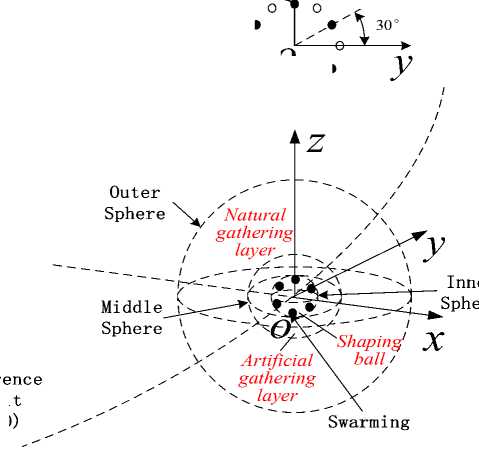
Secondly, according to the introduction of methodology in section II, by defining three spheres about target point, namely, outer sphere, middle sphere and inner sphere, and their radiuses meet the relationship: r outer '' r mdde ^ rimer , the region around target point can be further divided into three regions. From farthest to nearest, these regions are:

• 1)    Natural gathering layer , which extends from outer sphere (to middle sphere, as the name implies, g ^far is the main potential function. Thereinto, the outer sphere is the initial sphere of spacecrafts, where all spacecrafts are initialized with zero velocity; the middle sphere is set as an inner boundary of g ^far . However, it

should be noted that, according scenario introduced above, ^{g near} may be activated and instead of g ^far even when spacecraft do not arrive the middle sphere, here the running time of agent is beyond ^tnatural , a time parameter used to represent the biggest application duration of g ^far .

• 2)    Artificial gathering layer , it extends from middle sphere to inner sphere which is appreciably bigger than the circumscribing sphere of desired configuration. Similarly, ^{g near} is used here to continue the gather behavior. The name of this layer suggests that the trajectory of spacecraft is no longer a ballistic trajectory which is the classic trajectory in the natural gathering layer.

• 3)    Shaping ball , viz., the region enclosed with inner sphere, aiming to shape the final configuration by mainly using local potential l and ensure convergence by exploiting the artificial damping function ^d . Moreover, g ^planar and g ^phase usually be added to agree some demands in degree of freedom of configuration.

Thirdly, we assumed that each spacecraft not only knows itself coordinate and velocity at any time, but also can obtains the locational information in its sensing zone by on-orbit measurement or local communication, in simulation, the radius of sensing ball of spacecraft is Z r ; and the type of propulsion is continuous low thruster whose maximum acceleration is  umax

.

Moreover, in order to facilitate and reduce numerical error, parameters will be normalized in the following simulation, the normalization factors and public normalized parameters are listed in Table I and II respectively.

Table 1:		Normalization factors in simulation
Module	Parameter	Value	Meaning
	m s (kg)	1.9926 x 10 '26	Mass of carbon atom
Tersoff-Brenner module	l s (m)	1.315 x 10 ' 10	Equilibrium distance between carbon atoms
	e s (J)	1.0134 x 10 ' 18	Tersoff-Brenner potential well depth
	m e (kg)	5.9724 x 10 24	Mass of the Earth
	l e (m)	6.37813 x 106	Equatorial radius of the Earth
Space flight dynamics	<^, e ( rad/s)	7.2921 x 10 '5	Self-rotating angular velocity of the Earth
module	t e (s)	® - 1	Normalization factor of time
	v e (m/s)	l e / t e	Normalization factor of velocity
	a 2 e (m/s2)	ve / te	Normalization factor of acceleration

Table 2: Public normalized parameters in simulation

Module	Parameter	Value	Meaning
	M ( e )	1	Mass of agent
	R ( e )	1	Equilibrium distance between agents
	D ( e )	1	Potential well depth
	в	1.9725	Fitting parameters
	S	1.29	Fitting parameters
Tersoff-Brenner module	R (1)	1.95	Truncation distance
	R (2)	2.25	Truncation distance
	5	0.80469	Fitting parameters
	a 0	1.1304 x 10 -2	Fitting parameters
	c 0	19	Fitting parameters
	d 0	2.5	Fitting parameters
	to	1	Rotating angular velocity of GEO
	n	6	Number of spacecrafts
	l	10/ l e	Desire distance
	Z r	21/ l e	Radius of sensing ball of spacecraft
	u max	5 x 10-3/ a e	Maximum acceleration of thruster
Space flight dynamics module	desire	1.95 x 10 4 / t e	Ideal total time for reaching the center of the desired configuration
	t natural	0.975* desire	Time boundary of natural gathering layer
	x shift	0	the designed displacement of configuration in x direction
	r . outer	103/ l e	Radius of outer sphere
	r middle	102/ e	Radius of middle sphere
	T inner	15/ l e	Radius of inner sphere

Finally, after analyzing above, as a pilot research, this paper will take hexagon as the desired configuration and make a typical simulation with all degrees of freedom restricted: central position, orientation and phase of configuration. The center of final pattern is set at the origin of the reference frame o xyz , the plane of it is kept on the ^yz plane and phase angle is 30°(see

Fig. 1). It should be noted that as analyzed at the end of section II A, in order to verify the validity of our method in the cases of including large quantity of agents, we will only choose one target point as the center of dock potential filed although there are only six agents in our simulation).

Z Ч-<О Y O Earth Reference Orbit (GEO)

Dock       z Point Phase •           \ 30°   Angle ° А— 0 V > o y 0 е 0                 / / / / z / Outer Sphere       Natural gathering layer               y Inner Middle                            Sphere Sphere          o Shaping x Artificial     ball gathering layer Swarming Spacecrafts

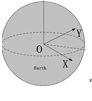
Fig. 1: View of simulation (not to scale). Black solid points represent the desired configuration with 30° phase angle, accordingly small circles in the top right corner denote the case of 0° phase angle

The usage of potential functions and other parameters except public ones in simulation are shown as follow in detail.

Table 3: The usage of potential functions in simulation

Behavior	Natural gathering layer	Artificial gathering	layer                 Shaping ball
Gathering	g far	g near ( g free )	g near g planar    g phase
Avoiding & Shaping	l	l	l
Dissipation	/	d	d
Table 4: Other parameters except public ones in simulation
Parameter	Value		Meaning
a f	5.1676 x 10 3		g free Amplitude coefficient of potential
k f	3.9822 х 10-10		Range parameter of potential   free
a pl	a f Equal to		Amplitude coefficient of potential planar
k pl	k f Equal to		Range parameter of potential   planar
ц	1.9926 x 10 -29		Amplification constant used in Eq. 14
^	2.4027 x 10 2		Dissipation coefficients
t all	4 х 104/ t e		Total time of simulation

And the corresponding results and analyses are given f ll

(a)

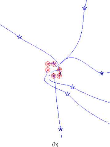
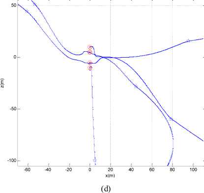
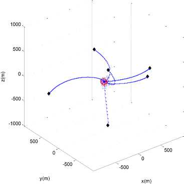
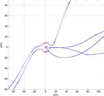
Fig. 2: Views of hexagon pattern simulation (Diamond: initial g free position of spacecraft; Pentacle: position of spacecraft when       is activated; Circle: stable position of spacecraft; Star: desired position of spacecraft; Solid line: path of spacecraft): (a) 3D view of far approaching phase; (b) 3D view of near approaching phase; (c) xy planar view; (d) xz planar view; (e) yz planar view

(a)

(c)

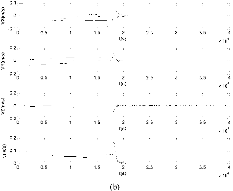
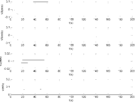
Fig. 3: Magnitude of velocity charts, where, v ^ (VX) ⁺ (VY) ^{+ (VZ} )   : (a)

during the first 200 s; (b) during the whole simulation procedure

(a)

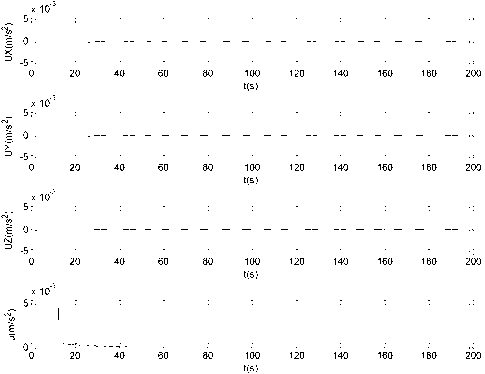
and then decelerated due to the combined effect of both g ^near , l and d to acquire the final position. The expensive phases of the whole procedure in terms of propellant consumption were the very first seconds, when the engines were constantly saturated to reach a ballistic trajectory (Fig. 4a), and the last part of the pattern shaping (Fig. 4b). During the simulation the magnitude of velocity of spacecrafts is less than 0.18 m/s, while the control acceleration is also not more than the allowed value as shown in Fig. 4. Moreover, the mean relative error of the mutual distance adjacent spacecrafts and the desire distance calculated based on the following formula.

N

X = [ZE(Il- j /1)]/(2N) iNi between l can be

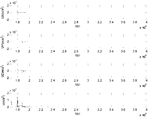
(b)

Fig. 4: Magnitude of control acceleration charts, where, u = V (UX ) + ^(UY) + ^(UZ ) : (a) during the first 200 s; (b) during the last 23350 s.

where i = ¹,²,—, N , N is the number of spacecrafts, Nⁱ is the set containing the closest neighbors of the i^th spacecraft and ^ij is the relative distance between the i^th and j^th spacecrafts at the final lattice acquisition time. In our case, the mean relative error is 0.0125. In fact, this error will become more and more small as time promote due to dissipation.

All above results and analysis show that our control strategy is available for the actual space mission. It should be noted that the scenario will be simpler than the one in simulation here if there is no demand on orientation or phase. Such as no orientation and phase demands, what should we to do is just keep local potential l and the artificial damping function d enabled in shaping ball, meanwhile the setting of natural gathering layer and artificial gathering layer keep unchanged. Moreover, agent sometimes will fall into the center of the desire configuration due to the particularity of Tersoff-Brenner potential filed which is an anisotropy potential model unlike the isotropy Lennard-Jones potential, but this is not allowed in a desired configuration without central agent such as our case. One of solutions is to fix a virtual agent with a new R ^{( )} (smaller than the desire distance ^l when interacts with other actual spacecraft agents) at the center of desire pattern.

In addition, our method cannot be only used to shape regular hexagon pattern, the structure unit of graphite ， but also regular tetrahedron pattern including central point, the structure unit of diamond( see Fig. 5). Of course, other patterns can also be shaped by using this method, such as equilateral triangle, square, regular pentagon and regular hexahedron etc., which are not included here for reasons of space.

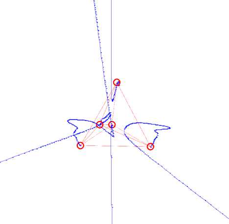
Fig. 5: 3D view of near approaching phase of regular tetrahedron configuration simulation (Circle: stable position of spacecraft; Solid line: path of spacecraft; Dash line: auxiliary line used to show the spatial structure of configuration; Dash-dot line: auxiliary line used to show the virtual covalent bond between “atoms”, i.e. spacecrafts).

• IV.    Conclusions

We have presented a new self-organizing and scalable control strategy for spacecraft swarm system in orbit around a planet, which allows agents to use limited sensor information and limited computational resources automatically form a desired pattern with the same mutual distance while avoid collision. Obviously, this method can be also used for other types of swarm, such as robots, unmanned aerial vehicles and unmanned submarines, etc. The method is based on the artificial potential field approach. Firstly, agents are gathered by a global potential field, which can be divided in two different parts, one far from the desired configuration, in which the gather behavior takes into account the gravitational force, and one close to the desired formation, in which space is considered to be flat. After that, the local lattice can be established by the local potential field. Here, we exploit the famous empirical many-body    potential-energy    expression    of hydrocarbons, i.e. the Tersoff-Brenner potential as the local potential field, so some interest configurations can be shaped, such as graphite and diamond lattices, etc. Finally, a viscous term was set to ensure converge.

Although other methods may have a simpler scenario for the simple hexagon lattice, such as Derek’s bifurcation method, the significance of our method is to validate the feasibility of using Tersoff-Brenner potential field for pattern formation in swarming spacecrafts. Analogously ， in our method, each agent only need to know their position, velocity and the position information of neighbors in their sensor ball during the formation procedure. That is, the method presented here has the following advantages:

• 1)    high robustness;

• 2)    low communication requirement;

• 3)    highly scalable.

Although the method has proven to be promising, further study and research is required. we will pay more attention on the following works: on the one hand, to try to use the method we developed to simulate large hydrocarbon molecules space structures in real space dynamic environment, such as the structure of diamond, graphene, carbon nanotube and fullerene etc., which will play important roles in the coming space swarm missions; on the other hand, to develop new swarm control technologies based on the latest achievements of molecular dynamic simulation, for example, try to use other new empirical potential field model. In short, we want to get more inspirations from the development of molecular dynamic simulation technology during developing the swarm control technology.

Acknowledgment

This research was funded by the Open Research Foundation of Science and Technology on Aerospace Flight Dynamics Laboratory of China (Grant No. 2012afdl023).