PD Controller Structures: Comparison and Selection for an Electromechanical System

Published Online January 2015 in MECS

The term control system design refers to the process of selecting feedback gains (poles and zeros) that meet design specifications in a closed-loop control system. The purpose of a control system is to reshape the response of the closed loop system to meet the desired response, the response depends on closed loop poles' location on complex plane [1] The available control system strategies and methods for control-system design are bounded only by one's imagination, there are many control strategies that may be more or less appropriate to a specific type of application, each has its advantages and disadvantages; the designer must select the best one for specific application, Engineering practice usually dictates that one chooses the simplest controller that meets all the design specifications. In most cases, the more complex a controller is, the more it costs, the less reliable it is, and the more difficult it is to design. Choosing a specific controller for a specific application is often based on the designer's past experience and sometimes intuition, and it entails as much art as it does science, [2].

Most design methods are iterative, combining parameter selection with analysis, simulation, and insight into the dynamics of the plant, [1,3]. An important compromise for control system design is to result in acceptable stability, and medium fastness of response, one definition of acceptable stability is when the undershoot that follows the first overshoot of the response is small, or barely observable, [1]. Beside world wide known and applied controllers design method including Ziegler and Nichols known as the “process reaction curve” method, [4-6]; many controllers design methods have been proposed and can be found in different texts including [1,7-11] , each method has its advantages, and limitations.

This paper focuses on PD controller and reviews it's main configurations, structures, modeling and most applied design techniques. The PD controller can be chosen, because of its simplicity, global stability, broadapplicability, also, it provides the ability to handle fast process load changes (e.g. in Pick and place robot), also PD controller reduces the amount of overshoot, [12].

• I.1    Controllers Configurations:

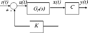
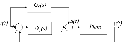
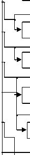
Most of the conventional design methods in control systems rely on the so-called fixed-configuration design in that the designer at the outset decides the basic configuration of the overall designed system and decides where the controller is to be positioned relative to the controlled process. The five commonly used system configurations with controller compensation are shown in Fig. 1, and include; ( a) Series (cascade) compensation , (b) Feedback compensation, the controller is placed in the minor inner feedback path in parallel with the controlled process. (c) State-feedback compensation the system generates the control signal by feeding back the state variables through constant real gains . (d)Series-feedback compensation a series controller and a feedback controller are used (e) Feedforward compensation: the controller is placed in series with the closed-loop system, which has a controller in the forward path the Feedforward controller is placed in parallel with the forward path, [12].

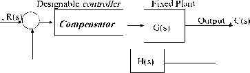
Fig. 1(a) series or cascade compensation and Components

Fixed Plant

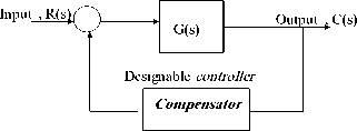
Fig. 1(b) Feedback compensation

Feedback

Fig. 1(c) state feedback

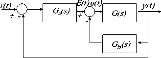
Fig. 1(d) Series-Feedback compensation (2DOF)

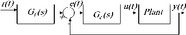
Fig. 1(e) forward with series compensations

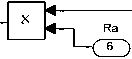
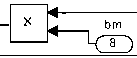
and analyze the open loop Robot arm system ,considering end-effecter is of cuboid shape, The total equivalent inertia, J equiv and total equivalent damping, b equiv at the armature of the motor are given by Eq.(2). To compute the total inertia, J_equiv , we first consider robot arm as thin rod of mass m , length ℓ , (so that m = ρ*ℓ*s ) , this rod is rotating around the axis which passes through its center and is perpendicular to the rod. The moments of inertia of robot arm and the cuboid end-effecter and can be found by Eq.(3). General torque required from the motor is the sum of the static and dynamic torque, assuming the robot arm is horizontal, that is, the weight is perpendicular to the robot arm, substituting arm and effecter inertias and manipulating, gives Eq.(3a). The robot arm has the following nominal values; arm mass, M= 8 Kg, arm length, L=0.4 m, and viscous damping constant, b = 0.09 N.sec/m. The following nominal values for the various parameters of eclectic motor used: V_in=12 Volts; J_m= 0.271 kg·m²; b m = 0.23 ;K t = 0.23 N-m/A ; K b = 1.185 V-s/rad; R a =1 Ohm; L a =0.23 Henry; T Load , gear ratio, for simplicity can be ,n=1. Potentiometer is a popular sensor used to measure the actual output robot (arm) position, θ L , potentiometer constant K pot =0.0667 to result in output angle of 180 for 12 V input.

G (s) = ^{6 (} s )

G ange ( s)   V in ( s )                                                   (1)

K t

{ [ ( L a J m S ³ + ( R a J m + Ь А ) S 2 + ( RX + KX ) S ] }

Fig. 1(f) Forward compensations

Fig. 1 commonly used system configurations with controller compensation[12]

b equiv

= b + b m    Load

II. Basic System Modeling and Parameters

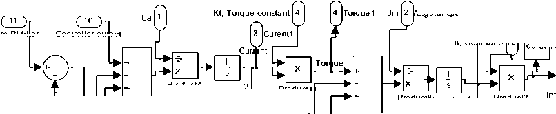
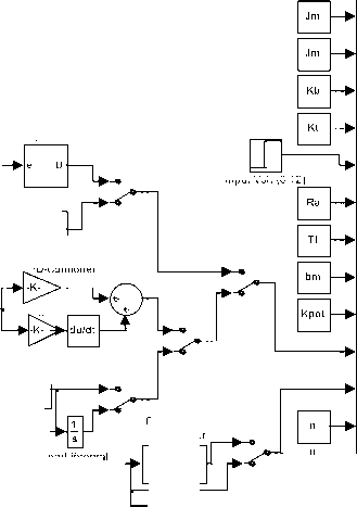
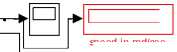
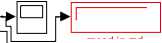
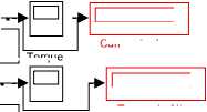
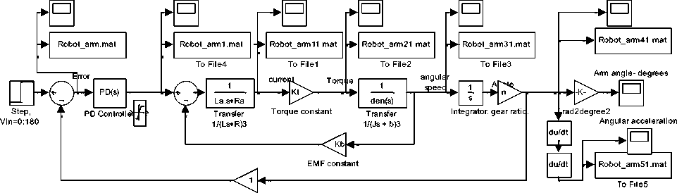
To test and compare forms and structures of PD controller, single joint robot arm is to be used as basic system. Because of the ease with which they can be controlled, systems of DC machines have been frequently used in many applications requiring a wide range of motor speeds and a precise output motor control [g-h]. Based on the Newton’s law combined with the Kirchoff’s law, the mathematical model of PMDC motor, describing electric and mechanical characteristics of the motor can be derived. In [16-17], based on different approaches, detailed derivation of different and refined mathematical models of PMDC motor and corresponding Simulink models, as well as a function blocks with its function block parameters window for open loop DC system motor selection, verification and performance analysis are introduced. The PMDC motor open loop transfer function without any load attached relating the input voltage, V in (s), to the motor shaft output angular motion, θ_m(s) , is given by Eq.(1) . Based on Eq.(1) and refereeing to[16-17] the Simulink models shown in Fig.s 2,3 are proposed.

There are dynamic requirements, which have to be satisfied depending on the motion and trajectories, where if fast motions are needed, these dynamic effects may dominate static phenomena, [13,15]. To model, Simulate

J - J J + J equiv     m     Load

N 1

N

l /2                               3

-l/2                       3

l/2    m    l3/8    1

= s 2=

-1/2   sl       312

J effector

T =

bh3

' bh3 + ML2'

+L (0.5 • M, • g • L + M2)

(3a)

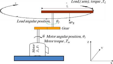
Fig. 2. Simplified schematic model of one DOF robot arm and DC motor used to drive arm horizontally [16].

Angular speed n, Gear ratio 12

Input Voltage

ter Controller output sJI

From PI fil

Product4 Integrator.2

Product1

ProductI8ntegrator..1

Product3

ter

T, Load torque

Sum.4

Product7 Sum.1

du/dt Derivative

Integrator..4

From i nput Volt to PI fil

Product10

Kb,

Product9

M F constant

Angular position

Product2

OUTPUT from summing to controller

angle feedback 9

Fig. 3 (a) DC machine subsystem model

L e ad or lag

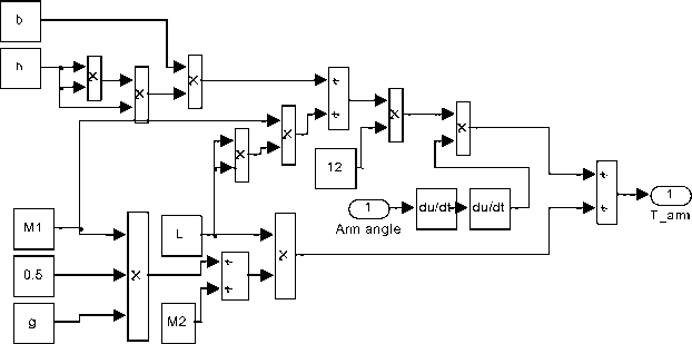
Fig. 3 (b) Robot arm torque Simulink model

PD-Fuzzy Controller

PID

> PID(s)

La

Jm

Kb, EMF constant

Kt, Torque constant

Input Voltage

Ra

T, Load torque bm

Kpot, Arm angle feedback

Controller output

From PI f ilter n, Gear ratio s+Zo s+Po

ZPD s+ZPD

Lead in` tegra comp.

Dead beat_ PD-prefilter

Input Volt (0:12)

PD-Controller

Robot Arm Subsystem

Angular speed

Angular position

Curent1

Torque1

Angular Acceleration

From input Volt to PI filter

OUTPUT from summing to controller

To File1

To File2

.

.

Angular speed.

speed in rad/sec

angular position.

speed in rad

Current.

Torque

Torque in N/m

Current in Amp

Angular acceleration

Angular acceleration Rad/m^2

Fig. 3 (c) Simulink models used to test PD algorithms

• III.    Mathematical Modeling Of PD Controller

Proportional plus derivative controllers take advantage of both proportional and derivative (rate) control modes. The control action of P-controller provides an instantaneous response to the control error, it pushes the system in the direction opposite the error, with a magnitude proportional to the magnitude of the error, P-controller transfer function is given by Eq.(4). A derivative controller differentiates the error signal to generate the controller output signal, the changing of the error indicates where the error is going to be in the future, that is predicting the error in future, based on the past and current state (e.g. slope) of the error, the derivative controller produces more control action if the error changes at a faster rate, D-controller transfer function is given by Eq.(5).

The D-controller action mainly works in transient mode, it has the effect of improving the stability of the system, and improving the transient response by providing a fast response to result in reducing the overshoot M p , settling time T S , small changes on both rise time T_R and steady state error E_SS , D-controller predicts, the large overshoot and makes the adjustment needed. In steady state mode: If the steady-state error of a system is unchanged, (constant), in the time domain, the derivative control has no effect, since the time derivative of a constant is zero. Both P and D terms of PD controller are fast, together will result in faster system.

G d ( 5 ) =

TDs aTs +1

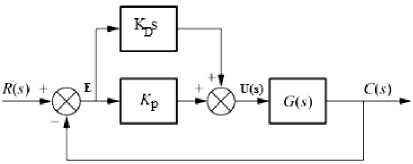
Fig. 4(a) PD controller arrangements

u (t )= Kpe (t )^U (5 )=E (5) Kp

G pd (s) = K p

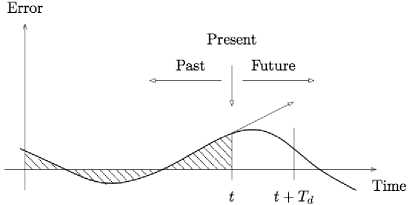
Fig. 4(b) PD action, [18]

u (t) = КDde(t) ^u(s) = kdS e (5) GpD (5) = KdS

• A.    Remedies for Derivative action; D-controller cascaded with a first-order low-pass filter

The D-term is not physically implementable, since it is not proper, also the D-term based on past and present states, extrapolates the current slope of the error (see Fig. 3), therefore has very high gain, this means a sudden rapid change in set-point (and hence error) will cause the derivative controller to become very large, also for high frequency signals would differentiate high frequency noise, and thus provide a derivative kick to the final control, this means for particular systems, the addition of D zero may cause overshoot in the transient response for the closed loop system and this is undesirable, since it can cause problems including instability. To solve this problem, and to implement D-controller, in processes with noise, the addition of a lag to the derivative term is applied by a pure differentiator approximation (Pure differentiator cascaded with a first-order low-pass filter, given by Eq.(6), with small time constant T, e.g. shorter than 1/5 of derivative time constant T D , where the larger the derivative time setting, the more derivative action is produced, if the derivative time is set too long, oscillations will occur and the control loop will run unstable. α is small number between [0.02:0.1], is recommended, this has the effect of attenuating (filtering) the high frequency noise entering the D-controller. Based on this, the derivative controller will have the form given by Eq.(7):

filter = —— ^ D filter =------ (6)

t s + 1        ^_        a T_Ds + 1

• B.    Proportional-Derivative, PD-controller

PD-controller controllers take advantage of both proportional and Derivative control modes, each of both is fast, both together are result in faster response, the output control signal of PD-Controller controller u(t), is equal to the sum of two signals (see Fig. 3(a)); The signal obtained by multiplying the error signal e(t) by K P and the signal obtained by differentiating and multiplying the error signal by gain K_D , as given by Eqs.( 5-8), taking Laplace transform for Eq.(8) and solving for transfer function, gives Eq.(9), Where : Z PD = K P /K D , is the PD-controller zero:

P        D dt      P (      KP dt J (8)

Gpd (5) = Kp + Kd5 = Kd (5 + KP) = Kd (5 + Zpd ) (9) KD

The transfer given by Eq. (9), shows that PD controller action properties are the both of P-and D-controllers, also, shows that PD controller is equivalent to the addition of a simple zero at Z PD = K P /K D , to the open-loop transfer function resulting in more stable system and improving the transient response, In the transient mode: PD -controller improves (speed up) the transient response, it will decay faster resulting in less settling time T_S , less time constant T , less peak time T_P , and reduced maximum overshoot M P. In steady state mode: PD -controller has minimum effect, from a different point of view, the PD controller may also be used to improve the steady-state error only when error changes with respect to time, because it anticipates the direction of large errors and attempts corrective action before they with large overshoot occur .

The main disadvantages are in that the PD controller, given by: C(s) = K P + K D s , is not physically implementable, since it is not proper, also D-controller, has very high gain, solutions are to approximate D-controller as lead compensator by the addition of pole, or by the addition of a lag to the derivative term, solves this problem, and the transfer function of a PD controller with a filtered derivative term is given by Eq.(10), where : T D :The derivative time is the time interval by which the rate action advances the effect of the proportional control action. N: With the range of 2 to 20, it determines the gain K_HF of the PID controller in the high frequency range, the gain K HF must be limited because measurement noise signal often contains high frequency components and its amplification should be limited.

• IV.    PD-Controller Configurations –A LGORITHMS

• A.    Series (cascade) PD-controller configuration.

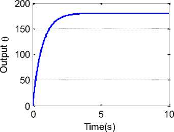
It is the most common control system topology, were the controller placed in series with the controlled process as shown in Fig. 4(a) , with cascade compensation the error signal is found, and the control signal is developed entirely from the error signal. Running Simulink model, for defined parameters will result in response curve shown in Fig. 4(b), PD parameters and response measures are shown in Table 2

Error                        Control                   Current           Torque              Angular speed                    Arm angle- Radians

Arm angle feedbacK

Fig. 5(a) Negative closed loop feedback control system with forward PD controller

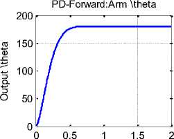
Time(s)

Fig. 5(b) Cascade PD-controller configuration

• B.    Rate feedback control configuration; D-term as rate feedback (feedback compensation).

The rate feedback controller is obtained by feeding back the rate of the output according to the block diagram given in Fig. 5(b). The rate feedback control helps to increase the system damping, decreases both the response settling time and overshoot [1]. In the case of rate (velocity) feedback, a portion of the output displacement is differentiated and returned so as to restrict the velocity of the output. Acceleration feedback is accomplished by differentiating a portion of the output velocity, which when fed back serves as an additional restriction on the system output. The result of both rate and acceleration feedback is to aid the system in achieving changes in position without overshoot and oscillation [19].

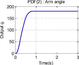
• a. Pseudo-Derivative Feedback (PDF) Control ;

Proportional rate feedback control

In 1977 Phelan [20-21] published a book, which emphasizes a simple yet effective control structure, a structure that provides all the control aspects of PID control, but without system zeros , and correspondingly removing negative zeros effect upon system response [22]. Phelan named this structure "Pseudo-derivative feedback (PDF) control from the fact that the rate of the measured parameter is fed back without having to calculate a derivative , PDF way of control is very simple and easily applicable, with main advantage that since the output value represents the result of several integrations, it will vary slower than the other signals in the system, and thus the differentiator’s response will be more realistic. The general form of closed loop transfer function, for system without any controller in the forward loop is given by Eq.(11). The closed loop transfer function, for rate feedback controller is given by Eq.(12), Comparing these two closed loop transfer functions, to find the relation between damping ratios result in Eq.(13), shows that the damping ratio is increased applying the rate feedback , and the undamped natural frequency is unchanged, resulting in improving transient response in terms of reducing in settling time and overshoot, and the derivative gain can be calculated as by Eq.(14), this means, based on damping ratio of original system closed loop transfer function without controller; we can design a rate feedback controller to achieve a desired damping[1],

^Tclosed ⁽ s )

^to n

^Tclosed ⁽ s )

5 2 + 2§tons + ton

to

s 2 + 2 (§ + 0.5Kr^ ) to„s + ton

^ Rate = § + 0.5 K

Kd = — ««-• ton

Rale ^ ll

- § ) K d = — (^ e - § ) ^to n

Fig. 6(d) Pseudo-Derivative Feedback (PDF) response for model in Fig.

4(d)

According to the block diagram given in Fig. 5(a), the closed loop transfer function is given by Eq.(15). As shown in Fig. 5(b)(c), for electric motor output angular position control, the measured output is angle and the rate of measured output angle is angular speed, which is to be fedback. If we place a tachometer, it will output a voltage proportional to angular speed, this can be feed back to the regulator. Tachometer-feedback control has exactly the same effect as the PD control, the response of the system with tachometer feedback is uniquely defined by the characteristic equation,

K_PG ( s )

_T           1 + G ( s ) K d S      ₌        K p G ( s )

^M   1 + G ( s ) K d s + G ( s ) K p   1 + G ( s ) K_Ds + G ( s ) K_p

1 + G ( s ) K_Ds

T ( s ) =------ ^{KpG (} s ) -----г

1 + G ( s ) ( K D s + K_p )

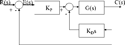
Fig. 6(a) Block diagram for PD-Controller with D-Controller as rate feedback

• C.    Decentralized PD approach

  Decentralized PD structure is shown in Fig. 6(a), the D-term is multiplied by velocity tacho-conversion constant Kc=0.02149 (V s/rad), and with unity feedback. In decentralized structure, also the desired output angle can be used as input signal with unity feedback, Running model for defined system parameters and desired output angle of 180, will result in output angular position response curves shown in Fig. 6(b), PD parameters and response measures are shown in Table 2.

whereas the response of the system with the PD control also depends on the zero at Z = -K P /K D , which could have a significant effect on the overshoot of the step response [1,23]. Running model in Fig. 5(c)(d) for defined system parameters, will result in response curves shown in Fig. 8, PD parameters and response measures are shown in Table 2.

Decentralized PD :Arm angle

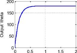
Time(s)

Fig. 7 Decentralized PD arm response

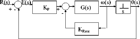
Fig. 6(b) Electric motor (robot arm) control

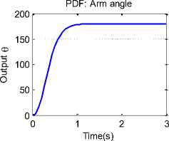
Fig. 6(c) Pseudo-Derivative Feedback (PDF) response for model in Fig.

4(c)

• D.    Design of PD-controller with deadbeat response.

Deadbeat response means the response that proceeds rapidly to the desired level and holds at that level with minimal overshoot. A deadbeat response has the following characteristics, (1) Steady-state error = 0, (2) Fast response; minimum both rise time T R and settling time T_s , (3) 0.1% < percent overshoot <2%, (4) Percent undershoot <2% (The ± 2 % error band). Characteristics (3) and (4) require that the response remain within the ±2% band so that the entry to the band occurs at the settling time T s [1,24]. the forward transfer function of DC motor system, with PD controller is given by Eq.(16). The system overall closed loop transfer function, T(s) , from input signal to sensor , potentiometer, output is given by Eq.(117):

Referring to [24], The controller gains K and K depend on the physical parameters of the actuator drives, to determine K and K that yield optimal deadbeat response, the overall closed loop transfer function T(s) is compared with standard third order transfer function given by Eq.(18), knowing that α =1.9, β =2.2 and ω Ts =4.04 are known coefficients of system with deadbeat response given by table 1, and choosing TS to be less than

2 seconds, gives Eq.(14). Calculating PD parameters and running model will result in response curve shown in Fig.

• 7,    PD parameters and response measures are shown in table 2.

^ ( s )                            p   D s   j^t

V n ( s ) "  [ ( L a J m ) s ³ + ( R a J m + b m L ) S ² + ( R . b m + KK ) S ]

_T       0(s ) ₌__________________________ ( K p + ^Kd S ) K_t __________________________

¹ ' V ,„ ( s )  ( L a J_m ) s ³ + ( R a J_m + b_mL a ) s² + ( R b  + K _tK_b + K d K ,K_pol ) s + K_pK,K_pol

G ( s ) =

^o 3 ³

s ³ + «to n s ² + Дю П s + оЗ

^ Ю *0.5 = 4.82, 4 ? = 4.82/2 = 2.41

,     ey_ ___________________ ( Kp + K d = ) Kt i ( l . J , ) ___________________

⁽ s ’ = V . ( s ) =     ( R , J , + b m L . ) , „ ( ^R a b . + KK b + ^K D ^K l ^K p.\Jp^Kp„

s +               s +                             s +

LJ am

LJ am

LJ am

K

D

K Kpo

o3 L J nam

K p

K Kpo

	Table 1. The coefficients of the normalized standard transfer function
System order	Optimal coefficients         Percent Overshoot   Percent Undershoot  Rise,90%   Rise,100%   Settling α    β    γ    δ    ε        OS%            PU%          T R        T R        T S
2nd	1.82                                    0.10 %                0.00 %             3.47        6.58       4.82
3nd	1.90   2.20                             1.65 %                1.36 %             3.48        4.32       4.04
4nd	2.20   3.50   2.80                      0.89 %                0.95 %             4.16        5.29       4.81
5nd	2.70   4.90   5.40   3.40               1.29 %                0.37 %             4.84        5.73        5.43
6nd	3.15   6.50   7.55   7.55   4.05         1.63 %                 0.94 %              5.49         6.31        6.04

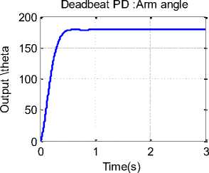
Fig. 7. PD controller arm Deadbeat response

• E.    Design of PD-con roller wi h prefil er.

Prefilter is defined as a transfer function GP(s) that filters the input signal R(s) prior to calculating the error signal. Adding a control system to plant, will result in the addition of poles and/or zeros, that will effect the response, mainly the added zero, will significantly inversely effect the response and should be cancelled by prefilter, therefore the required prefilter transfer function to cancel the zero is given by Eq.(19). In general, the prefilter is added for systems with lead networks or PI compensators. A prefilter for a system with a lag network, mainly, is not, since we expect the effect of the zero to be insignificant[25], running model with deadbeat design with prefilter added with ZPD= 5.1841, will result in response curve shown in Fig. 8, PD parameters and response measures are shown in Table 2.

PD with Prefilter: Arm angle

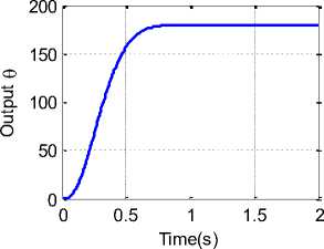
Fig. 8. PD-Controller design for deadbeat response with prefilter.

Comparing response curves shown in Fig. 6 and Fig. 7, show that the negative characteristics are eliminated (smoothed) and the system response is speed up.

Gpr efiiter (s) = _, Where : Z pd = K P ^{(19) (}s + Z pD ) K_D

• F.    PD control design with both position and velocity feedback.

The feedback system structure is shown in Simulink model given in Fig. 9(a), a velocity feedback is used to stabilize systems that tend to oscillate, for this system the output is the angular displacement, θL, the rate of change of angular position, dOL (5 ) / dt , is the actual output angular speed, and the error signal , Ve ,is given by Eq.(20), talking Laplace transform, and separating gives Eq.(21). Running model for defined system parameters with Ktach =0.6 and desired output angle of 180, will result in response curves shown in Fig. 9(b). Running model will result in response curve shown in Fig. 7(b), PD parameters and response measures are shown in Table 2.

V e = V n - K po_t 6 o — K tac   °"             (20)

dt

V e ( 5 ) = V n ( 5 ) - L ( ( 5 ) ( K pot - ^S )       (21)

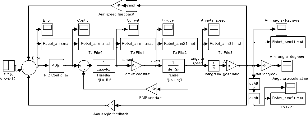
Fig. 9(a) PD control of robot arm output position with both position and velocity feedback

Position and Velocity: Arm angle

G Lead ( 5 ) = K p + ^ —

5 +J

_ Kp (5 + P ) + KdP5

5 += ( Kp + KdP ) —

KPP kp + kdp

5 + P

Now, let K_c = K_p + K_DP and z =

Fig. 9(b) PD response with both position and velocity feedback

G. Approximated PD Controller: Lead compensator.

Since PD controller given by Eq.(9) , is not physically implementable, since it is not proper, also PD controller would differentiate high frequency noise, thereby producing large swings in output. to avoid this PD-controller is approximated to lead controller of the form given by Eq.(22)[1], rearranging Eq.(22) gives Eq.(23):

Ps

G pD ( 5 ) * G Lead ( 5 ) = K p + К-

5 + P

^K P ^P k_p + k d p

we

obtain the approximated PD controller transfer function given by Eq.(24):, and called lead compensator Where Z o , P o compenstaor zero and pole respectively, and Z o < P o , the Z o is closest to imaginary axis and the larger the value of P o the better the lead controller approximates PD control. Lead compensator is applied using series controller configuration. Running model with lead compensator, will result in response curve shown in Fig. 10, Lead compensator parameters and response measures are shown in Table 2.

GLead (5 ) = Kc

5 + Z°5 + P°

Lead Compensator : Arm angle

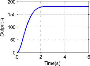
Fig. 10. Lead compensator responses

• H.    Lead integral compensator

Lead integral compensator transfer function is given by Eq.(25), it is used to eliminate steady state error, but the transient response settling time and overshoot may become large, a also the system may be subject to instability problems as the controller gain increased. Running model with designed Lead integral compensator, will result in response curve shown in Fig. 11

G Lead _ Integral ⁽ s )    ^KC

s (s + Po ) Cs (s + Po )

Fig. 11 Lead integral compensator response

• I.    Fuzzy-PD , FLPD-Controller,

Fuzzy logic control FLC is a control method based on fuzzy logic, which can be described simply as ’’control with sentences rather than equations’’ [26]. One of the most important advantages of fuzzy control is that it can be successfully applied to control nonlinear complex systems using operator experiences or control engineering knowledge without a mathematical model of the plant. As shown in Fig. 12(a), the general structure a

FLC constitutes of four principle components: fuzzification interface, knowledge base, decision-making logic and defuzzification interface [26-28]. FLC is applied using series controller configuration.

A FPD controller is a fuzzified proportional-derivative ( PD ) controller. It acts on the same input signals, but the control strategy is formulated as fuzzy rules. The FPD controller has three gains, which are mainly for tuning the response, and they can also be used for scaling the input signal onto the input universe to exploit it better, where the crisp proportional derivative controller has only two gains which make it flexible and better. A typical structure of FPD controller is shown in Fig. 12(b). It has two inputs; the error signal ‘ e ’ and the change of the error ‘ de/dt ’. The first input will be transformed from value ' e ' into the value ' E ' after multiplication with the error gain K_Error [26,28], as given by Eq.(26). By the same procedure, the second input will be transformed from value ‘ de/dt ’ ' into the value 'DE' after multiplication with the change of error gain K D_Error as given by Eq.(27). The two fuzzy inputs ' E ' and 'DE' are processed by the rule base stage to produce the a new fuzzy variable 'u' which will be transformed into the value ' U ' after multiplication with the output gain K U as given by Eq.(28), bases on this, the control signal U(n), is a nonlinear function of error and change in error as given by Eq.(29),

Considering that the function f is the rule base mapping, with two inputs and one output, and the defuzzification method must be “centre of gravity”, the output of function f of Eq.(29) will approximate the sum of two inputs, and manipulating to result in Eq.(30), now comparing the ideal PD transfer function given by Eq.(5) and Eq.(23), the gains are related as given by Eq.(31)[28].

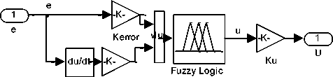
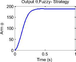
The design procedure of fuzzy PD controller based on linear PD controller as given in [28], is accomplished as follows: (a) find the best linear PD controller gain (in our case given in Table 2 K P= 3792.14 and K D =0974.19 ,), (b)Determine maximum error, (c) Determine the error gain K_Error : (in our case, the magnitude of the maximum error is 12, therefore the error gain will be equal to 12), (d) Compute the output gain K_U , by Eqs.(31), (e) Calculate the rate of error gain by Eqs.(31), (f)design Fuzzy PD controller. Fuzzy PD control structure in Simulink is shown in Fig. 12(c). Running model with designed FLC ,will result in response curve shown in Fig. 12(d).

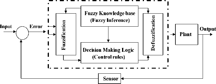
Fig. 12(a) The general structure a fuzzy logic controller (FLC)

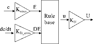
Fig. 12(b) Fuzzy PD control structure

E = е-Кг

Error

de

Controller

Kderror

Fig. 12(c) Fuzzy PD control structure in Simulink

D Error dt     ^_

U = u • Ku			(28)
„ .            de _ U = f ( e • K Er ,     • K d Error ) • u • K u dt _			(29)
u = ( e • KB „ + de • K d dt de K D _ Error = (e +     •      _      ) • u • dt Error	) • u • _ Error KuKError	K u	(30)
v ^           de ( t ) ) /    de e • K   e ( t ) + T          = ( e +--- P v        D dt J        dt K p = K u ' Ke™, K D _ Error	k" _ KD _ Error --_—) • u K Error	■K u   Error	(31)
TD   K K Error

K D = K u ■ K d _ Eror

Fig. 12(d) PD-FLC, PD Fuzzy Controller response

Table 2

Configuration		K P	K D	M P	5T	DCgain (≈)
PD Forward		3792.14	0974.19	-	0.6	179.999 ≈ 180
PD PDF		3785.530047	50	-	1.1	179.9995 ≈ 180
Decentralized PD		20945766.175565		-	0.7	179.95
PD with Position & Velocity feedback		2140951.93	365072.3	-	3.5	180
PD with Deadbeat response		3 4161	21094	0.2	0.9	180
PD with prefilter		5753.37	1109.79	-	0.7	180
Lead compensator		K=18000, Z o = 100, P o = 2000		-	2.2	180
Lead integral Comp.		K= 10500, Z o = 0.01, P o = 14		-	3	180
Fuzzy-PD	K Error =0.0099	K D_Error = 35714	K u =12000000	0.2	0.4	180

• V. Conclusions

PD controller modeling, configurations and control algorithms are linear control problem due to the complicated relationship between its components and parameters. The research that has been carried out in PD control systems covers a broad range of issues and challenges. Many different control methods for PD controllers have been developed and research on improved control methods is continuing. Most of these approaches require system models, and some of them cannot achieve satisfactory performance under the changes of various road conditions. While soft computing methods like PD Fuzzy control doesn’t need a precise model. A brief idea of how soft computing is employed in DC motor control is given.