Peculiarities of using 2D electrical resistivity tomography in caves

Geophysical methods are widely used in archaeological studies (Campana, Piro, 2008; Witten, 2017; El-Qady, Metwaly, Drahor, 2019). One of the important questions that could be answered with geophysics is: how deep is a bedrock. Precise information about bedrock’s form and deepness can bring a vast improvement to excavation planning. Electrical resistivity tomography (ERT) is an effective method for such studies. Bedrock and sediments are often quite different in their electrical resistivity; therefore, the bedrock’s surface can be registered as a high-contrast border in an electrical resistivity section. In the case of irregular surface of bedrock, three-dimensional ERT is required to build a correct model of it. The situation inside a cave is more complex: long and narrow space gives no opportunities to implement a 3D survey. Beyond that, the electrical current can flow through the cave ceiling and make an unexpected contribution to measured data. We have found two articles where ERT studies inside closed space are considered: in a pyramide (Tejero-Andrade et al., 2018) and in a church (Tsokas et al., 2008). Most often, geophysical studies are carried out above caves, on the daylight surface, for establishing the location of passages or the stability of the cave’s roof (Leucci, De Giorgi, 2005; Cardarelli et al., 2010; Martinez-Moreno et al., 2013). An ERT application for determining of sedimentary layer thickness and morphology was described, whose functions included prospecting sites of archaeological interest. Depth of electrical resistivity sections did not exceed 4 meters, whereas archaeological excavation showed 12-meter thickness of sediments (Obradovic et al., 2015).

The problem turned up for the authors during multidisciplinary research at Selungur Cave, in the southern part of the Fergana Valley, in Kyrgyzstan (Fig. 1). This cave is one of the largest karst cavities

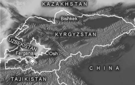
Fig. 1 . Location of Selungur Cave.

in Central Asia. The site was excavated in the 1980s, when it was described as an Early Paleolithic item. New study in 2014 has proved that stone complexes from Selungur Cave have Middle Paleolithic characteristics (Kolobova et al., 2018; Krivoshapkin et al., 2018). The scientific significance of the site, due to the uniqueness of its anthropological and archaeological finds, requires further research into it.

Methods

Geophysical methods, including ERT (Tsibizov et al., 2017), were used there in order to choose the most promising areas to excavate. Electrical resistivity tomography was performed using the “Skala-48” equipment along 6 parallel profiles located at a distance of 1 m from each other along the main gallery of the cave (Fig. 2, a ). A pole-dipole array was used for measurements (Fig. 3). It is more sensitive to local inhomogeneities, as compared to the Wenner-Schlumberger array, and the data obtained are less noisy as compared to the dipole-dipole array. The number of electrodes was 48, the distance between the electrodes varied from 1 to 5 m, and the n factor varied from 1 to 6. The maximum na distance was 30 m. The maximum depth of research was 11 m. In order to decrease grounding resistance, points of contacts were watered with brine.

Data processing was carried out using the twodimensional and three-dimensional inversion programs Res2DInv and Res3DInv (Loke, 2002, 2007). A robust inversion with a standard threshold coefficient of 0.05 was used. This limitation tends to give a model with contrasting boundaries between areas with different resistance values, but within each area these values are almost constant. This is acceptable for solving such a geological problem as the boundary between loose and bedrock rocks, which corresponds to our case.

Results

In the lower part of the geoelectric section in profile 4, the estimated boundary of the top of the bedrock with a specific electrical resistivity of 600– 2000 Ohm∙m was identified (see Fig. 2, b ), overlaid with loose deposits (200–500 Ohm∙m). Sediments with a resistivity of less than 100 Ohm∙m in the interval 25–30 and 35–40 m are represented by moist cave loess. Large fragments of the roof buried in loose rocks are distinguished by high-resistivity anomalies.

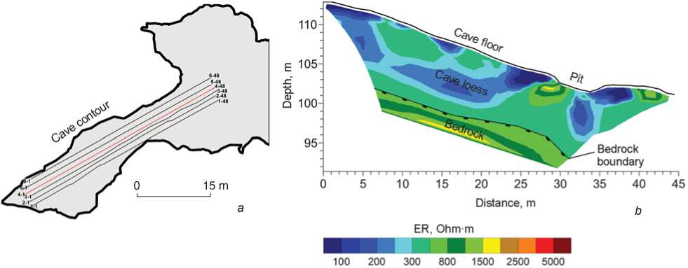
Fig. 2 . Location of profiles inside Selungur Cave ( a ), and resistivity section along profile 4 ( b ).

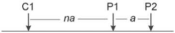
Fig. 3 . The scheme of pole-dipole array: C1– current electrode; P1, P2 – potential electrodes.

An area of a collapse appears on the section as a local anomaly of high resistivity in the interval of 41–43 m. Starting from 30 m, the bedrocks subside abruptly. This is explained by a fault zone that cuts the cave across the main gallery prolongation. The results of electrotomography have been confirmed during excavations: the depth of the sediments in the largest gallery of Selungur Cave reaches 6–9 meters.

The obtained results seem quite informative; nevertheless, it is not clear how trustworthy they are. In order to clear up this question, we conducted numerical modeling of ERT surveys in caves with different geometrical parameters. Synthetic results were analyzed and compared to field data.

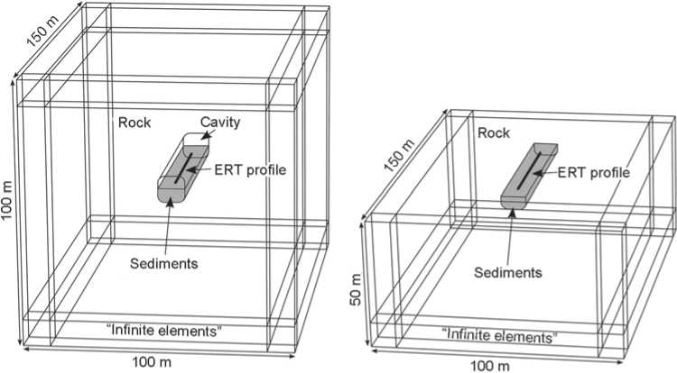
Numerical modeling was done with Comsol Multiphysics software. The cave was approximated by a 3D-medium (150 × 100 × 100 m) with a cavity partially filled with sediments (Fig. 4). The length, width, and height of the cavity’s free space were equivalent to 70, 10, and 5 m respectively. The thickness of the sediments varied between 2.5, 5, and 10 m. The electrical resistivity of the medium was estimated during the field studies (Tsibizov et al., 2017) and equivalent to 1000 Ohm∙m for the bedrock and 200 Ohm∙m for the loose deposits. In order to estimate the influence of the ceiling (which could conduct a part of the current), all numerical experiments were carried out in models both with ceiling and without it (half-space models). A pole-dipole array was modeled (according to the field measurements). The model was enclosed by “infinite elements” (to model the infinite electrode) with “ground” conditions (U = 0) on their external boundaries. On the basis of the modeled data, two-dimensional inversion was done with RES2DInv software. The number of data points for each profile in 2D-modeling was 916. In Fig. 5–7, inversion results in six considered cases are provided.

With the sedimentary layer 2.5 m thick (Fig. 5), the thickness of the sediments is determined quite adequately. In the first case (without a roof), a false low-resistivity anomaly (up to 300 Ohm∙m) appears starting from a depth of 12 meters. Inversion yields a bedrock resistivity bigger by a factor of 2–5 than in the forward model. In the second case (with a roof), similar results are obtained, but the low-resistivity anomaly reaches 150 Ohm∙m and starts from a depth of 9 m.

With the sedimentary layer 5 m thick (Fig. 6), the thickness of sediments in these both cases is underestimated (3.5 m), and bedrock resistivity is twice as big as in the model. Low-resistivity anomaly (up to 550 Ohm∙m) is recorded only in the second case (with roof).

With the loose deposits 10 m thick, the surface of bedrock cannot be determined if the cave’s wall is 5 m from the profile (Fig. 7). The wall creates a false “border” in the section at a depth of 5 m. Bedrock resistivity is restored quite well (1200 Ohm∙m) in the model with a roof; and in the restored half-space model without roof, it rises up to 4200 Ohm∙m with depth, which is not in agreement with the true model.

а

b

Fig. 4 . General view of the considered finite-element models.

a – cavity with low-resistive (200 Ohm∙m) sediments inside conductive (1000 Ohm∙m) space; b – conductive half-space with sediments.

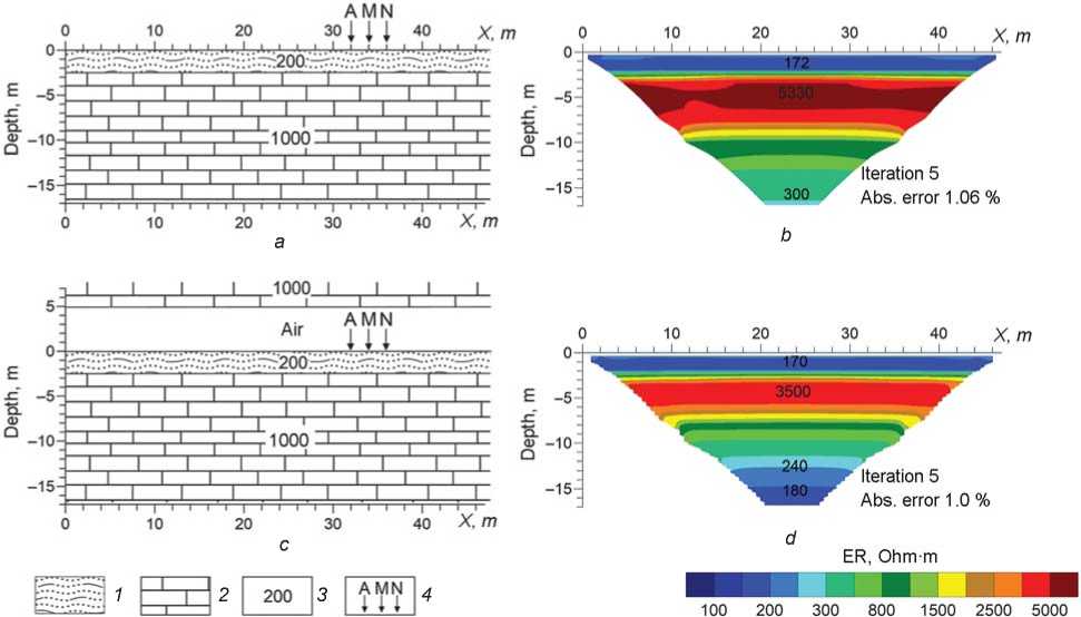
Fig. 5 . Geoelectrical models of cave without roof ( a ) and with roof ( c ), and the respective 2D inverse model resistivity sections ( b , d ) of forward modeling data. Thickness of sedimentary layer is 2.5 m.

1 – cave loess; 2 – limestone; 3 – resistivity; 4 – pole-dipole array.

Discussion

Numerical modeling showed that 2D automatic inversion that uses a forward problem for half-space cannot be applied for processing of data obtained from the cave in the general case. The sedimentary layer’s thickness will not be determined if it exceeds the distance to the cave’s wall. The electrical resistivity of sediments and bedrock will be determined incorrectly.

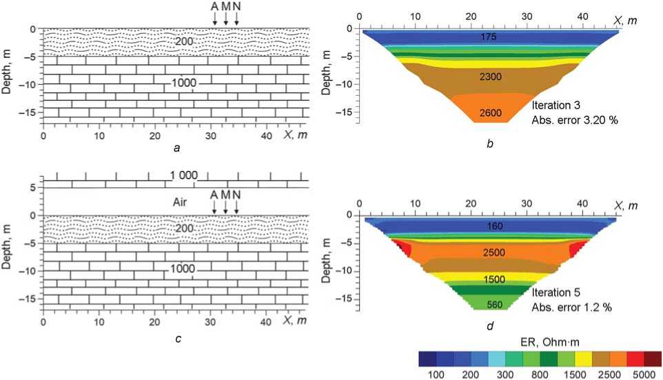
Fig. 6 . Geoelectrical models of cave without roof ( a ) and with roof ( c ), and the respective 2D inverse model resistivity sections ( b , d ) of forward modeling data. The thickness of sedimentary layer is 5 m.

See Fig. 5 for conventions.

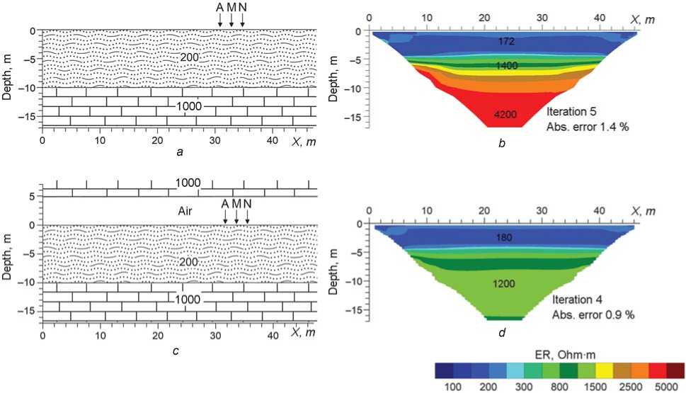
Fig. 7 . Geoelectrical models of cave without roof ( a ) and with roof ( c ), and the respective 2D inverse model resistivity sections ( b , d ) of forward modeling data. Thickness of sedimentary layer is 10 m.

See Fig. 5 for conventions.

Additionally, a three-dimensional survey was modeled in order to estimate how such a setting could improve the results. Seven parallel 2D survey lines were combined into a 3D set (Fig. 8). Data from profiles 2, 3, 4 were used twice—for these and for symmetric profiles (which are not shown in the Figure). For the subsequent inversion, Res3DInv software was used. Outer profiles were set on the cave wall. The total number of measurement points in 3D modeling was 6412.

In the case of low (2.5 m) thickness of sediments (Fig. 9, a ), the bedrock-sedimentary border is determined confidently; but the resistivity of

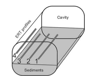
Fig. 8 . Scheme of ERT profiles in three-dimensional modeling.

sediments (120–130 Ohm∙m) and bedrock (up to 2250 Ohm∙m) is under- and overestimated, respectively, as compared to the true model. In the case that the sedimentary layer’s thickness exceeds half of the cave’s width (Fig. 9, b), neither bedrock depth nor resistivity of the layers can be restored. The depth of the border between low- and high-resistivity layers (sediments and bedrock) was higher than in the geoelectrical model of the cave. As can be seen from the above, even three-dimensional inversion does not restore the geoelectrical model of the cave in examined cases.

Do the results mean that for each cave wrong geoelectrical sections would be obtained? The field data reject this. The section does not contain any low-resistivity anomalies in its lower part (see Fig. 2), but the sedimentary layer’s thickness (8 m) is bigger than half of the cave’s width (5 m). Why do the modeling results contradict the field data? We supposed that the complex geometry of the cave was not taken into account, and built another model (Fig. 10, a ): cave walls were extrapolated downwards (in accordance with the observed slope angle of 70° in their exposed part), and a rough form of the roof was also included in the model. The sedimentary layer’s thickness was assumed to be 8 m, its resistivity 200 Ohm∙m, and bedrock resistivity 1000 Ohm∙m (according to field data). The line was situated along the cave, equidistantly from its walls.

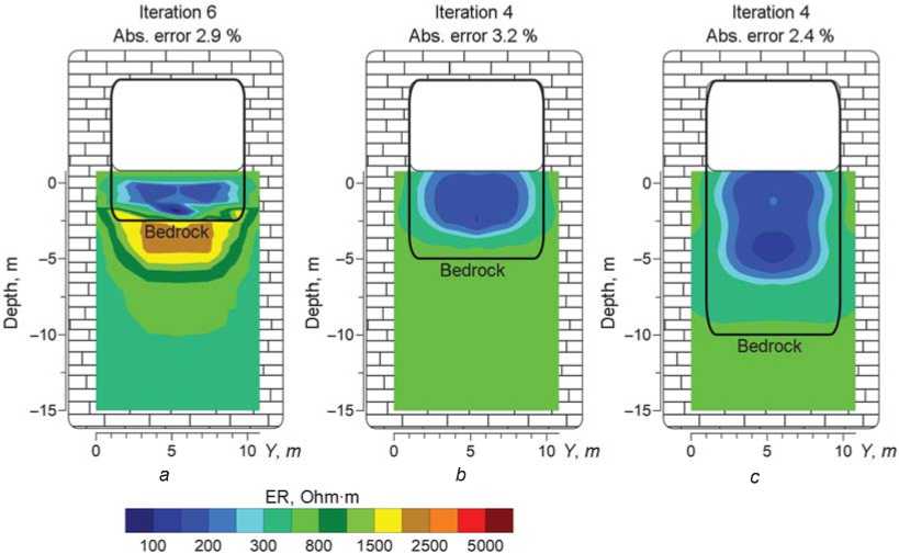
Fig. 9 . 3D restored model resistivity sections with thickness of sediments 2.5 m ( a ), 5.0 m ( b ), and 10 m ( c ).

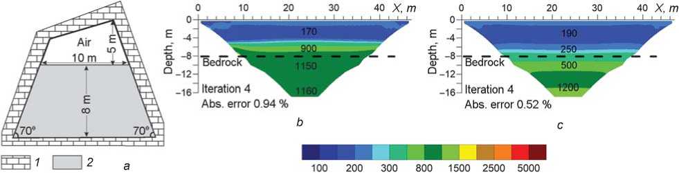
Fig. 10 . Model of Selungur Cave with sloping walls ( a ), and inversion results for this model ( b ) and for simple two-layered model ( c ).

1 – bedrock; 2 – sediments.

The three-dimensional forward problem was solved for the model, and then, on the basis of the obtained data, two-dimensional automatic inversion (developed for half-space) was done. In this case, the inversion yielded a good-fitting result: resistivity and border are restored (Fig. 10, b ). We compared the obtained data with the inversion result for a two-layered model with similar parameters (ρ₁ = 200 Ohm∙m, h ₁ = 8 m, ρ₂ = 1000 Ohm∙m, h ₂ = ∞). The resistivity of the upper layer is quite close to “real”, but the border is diffused (Fig. 10, c ). We have assured that in the case of diverged walls their influence on the current distribution was smoothed over, and two-dimensional inversion for half-space yielded a credible result.

Conclusions

ERT with the use of 2D inversion generally cannot be applied to study inside a cave whose half-width is smaller than the thickness of sediments. Use of the method under adverse conditions can lead to the production of false low-resistivity anomalies in the lower part of the section, error in locating of borders of rocks, and incorrect estimation of their electrical resistivity. Three-dimensional survey and inversion do not essentially improve the quality of results. Nevertheless, in some cases (as was shown from the abovementioned field study), two-dimensional ERT gives a good-fitting model of cave structure. This becomes possible when cave walls diverge, with the depth and current distributed approximately as in 2D medium. The use of other geophysical techniques, such as ground-penetrating radar, in complex with ERT seems efficient, but can be complicated by reflections from caves’ roofs and walls.

Acknowledgements

This study was supported by the Russian Foundation for Basic Research (Project No. 17-29-04122). The authors express their deep gratitude for the invaluable help of students from Osh and Batken State Universities in the course of fieldwork.