Performance Analysis of a System that Identifies the Parallel Modules through Program Dependence Graph

Published Online September 2017 in MECS

Despite Moore's law [3], uniprocessor clock speeds have now stalled, rather than using single processors running at ever-higher clock speeds, and drawing ever increasing amounts of power, even consumer laptops, tablets and desktops now have dual, quad or hexa-core processors. Job Scheduling on parallel computer [21] or parallel machines has been an imminent topic in the past couple of decades. Many researchers are working to invent optimization techniques for scheduling multiple jobs on parallel machines. So researchers started thinking parallel [13] to achieve good performance of applications and co up with technological growth reflecting in day-to-day life. One approach is to parallelize a program [9] is to rewrite it from scratch. However, the most common way is to parallelize a program incrementally, one piece at a time. Each small step can be seen as a behavior preserving transformation, i.e., a refactoring Programmer prefer this approach [4] because it is safer; they prefer to maintain a working, deployable version of the program. Also, the incremental approach is more economical than rewriting. For our approach we consider input as Abstract Syntax Tree i.e., The Abstract Syntax Tree (AST) [5] is a representation of the source code that is commonly used in compilers. It gives complete representation of the source code in the sense that it is possible to re generate an equivalent version of the original source code from an AST. The only things that are not modeled by an AST are spaces, blank lines and comments. The AST is closely related to the parse tree and hence to the formal grammar of the programming language. The only difference with the parse-tree is that the AST usually removes useless constructs, such as useless parentheses. The rules on what and how useless constructs are removed are not clearly defined and vary from one implementation to another.

The PDG [19] is constructed for the AST in the preceding step, which procreate perspicuous twain the data and control dependences for each operational statement in a program. Data dependence graphs have sustained some optimizing compilers [11] with a definite effigy of the definition-use relationships inherently commenced in a source program [6,7]. A control flow graph [8] is a conventional embodiment for the control flow interconnections of a program; the control conditions on which an operation depends can be described in a graphical form. The program dependence graph extraordinarily denotes both the essential data relationships, as present in the data dependence graph, and the important control relationships, without the unwanted sequencing present in the control flow graph. These essential dependences determine the necessary sequencing between operations, producing potential parallelism. Approachability of statements in a program can be determined by using reachability definition algorithm and also demonstrated through an example and Finally a new approach where even topological sort is used to find nearest predecessor which has been demonstrated algorithmically as well as with example and its computational time is also calculated and graphically depicted.

• II.    Construction of PDG

The primary dominion of graph transformations [14] in inured is that they effete a mannered and mathematical model that capitulate for divergent cursory fortuitous upon abilities, umbrella of the aptitude prone to a given transfiguration is remedy. Flow analysis is a technique of analysis of data and control flows of a source program. In object-oriented programming languages [1], preconditions [15] can be established by the data flow in source program i.e., the extracted method is acknowledged with at most one result and the control flow in a program conciliate whether the method can be extracted at all or not i.e., it has to verify that there must be a unique entry and unique exit precondition scrap. Program Dependence Graph (PDG) is a figurative illustration [2] of a program moiety, which has a docility of representing both control and data dependences between different segments of program. Control dependences mediates next instruction to be executed and data dependences pageant the value ascribe to variable ‘a’ in statement ‘X’ is recycled in other sections in a program. The construction of PDG consists of two steps, initially construct Control Dependence Graph (CDG) for an Abstract Syntax Tree (representation of a program segment) and secondly incorporate data dependencies to CDG using reachability algorithm.

• A.    Abstract Syntax Tree (AST)

An AST is a non-linear data structure, hierarchical representation of the abstract syntactic anatomy [5] of source code drafted in a programming language. Each node of the tree signifies a construct occurring in the source code or every individual statement represented as a node and it is widely targeted in syntax analyzer phase of a compiler. In other words it is basically represents the structure of code. Abstract syntax trees are data structures extensively employed in compiler design, due to property of personify the representation of program code. The generation of AST is an output of syntax analyzer, which is a second phase of compilation. It recurrently oblige as an intermediate representation of the program through multiple phases that the compiler expects, and has a great role in the determination of targeted production of the compiler.

It provides abstract view of a given source code and first node (root) is main_node, it has eight Children to represent S1 to S6 statements, Predicate P1 and statement S10. The while loop has three children one for condition inside while, second for if_else and one for S9. The conditional construct if_else has further has three links one for it’s own condition, one for if_clause and one for else_clause. The construction of AST is shown here for the given below segment.

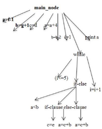
Fig.1. Program with AST

Program segment:

SI: a=f-l

S2:b~g+1

S3: c=d

S4: a=a+4

S5: b=b-2

• S6:    i=l

Pl: while (i<=5)

P2:     if(a

• S7:     c=e

• S8:     a=c+b

• S9:     i=i+l

S10: print a

• B.    Construction of CDG

CDG is Control Dependence Graph, which reflects control dependences between different segments of a program. If a statement ‘A’ has control dependence on statement ‘B’, then ‘B’ has to be executed priory as compared to ‘A’. In this section, we have demonstrated our approach with an algorithm and as well as with an example. The CDG construction takes Abstract Syntax Tree (AST) as an input and Produces Control Dependence Graph (CDG) as an output. To maintain simplicity in explanation, we consider structured control statements i.e., while and if_else, simple assignment statements, unconditional transfer of control statements i.e., goto statements and so on. To implement our approach we used data structure Stack and it’s operations PUSH and POP to insert and delete an element from the stack to maintain nesting and control dependences between the modules of a program. To have access on each and every statements of AST, preorder traversal (root, left, right) is done. Algorithm begins with construction of entry node, which denotes entire process is created and placed in STACK, subsequently nodes are added to the STACK, the children of the nodes are at the top of the STACK. Once innermost statements on the top of the STACK get evaluated, then next level of the statement will be evaluated. For example if_else statement in placed inside the while loop, node will be added as active or live for if_else, once it is evaluated then control moves to the while statement.

Whenever there is a conditional constructs in program, one region node is created with the name Ri, it has further child link to predicate node (Pi), which in turn denotes the conditional statement. As Pi is a conditional statement, it has two children links one for true and other for false, again two region (body) nodes will be created for true and false clauses of predicate node, under these region nodes the corresponding statements will be evaluated. Through backward arrows repetition of statements under looping constructed are handled and these backward arrows will be connected to the entry of that region node (Ri).

Algorithm:

Algorithm CDG_construction( T, root[T])

// T is abstract syntax tree; root [T] is address of T.

//This algorithm takes AST of a program S as input and produces CDG as output for the program S.

//For implementation the PUSH and POP operations on the data structure STACK (ST) is performed.

//main_node is nothing but root[T]

{ while ( nodes are present in AST) do

{ node=call CDG_Insert_Node( );

switch( node)

{ case main_node:

{ node=call CDG_Insert_Node(entry,live );

consider node as root of CDG

PUSH(ST,node);

Create an exit node for latter use;

} case ‘=’:

{ node=call CDG_Insert_Node(statement, live );

} case ‘while’:

{//beginning of while node=call CDG_Insert_Node(head, live);

PUSH(node);

node=call CDG_Insert_Node(predicate,node );

node=call CDG_Insert_Node(body,predicate );

PUSH(node);

// end of while; condition id false node=POP(ST)

solve the statement in ‘node’ node=POP(ST)

this will be the header node, i.e. the body of while loop is executed node=call CDG_Insert_Node(statement followed by while,live );

consider node as Top of the stack

} case ‘if_else’:

{ node=call CDG_Insert_Node(predicate,live );

PUSH(ST,node);

Begin if_clause(true)

node=call CDG_Insert_Node(body,live );

PUSH(ST,node);

Begin else_clause(flase)

node=call CDG_Insert_Node(body,live );

PUSH(ST,node);

End of if_else

Node=POP(ST);

Solve the statement in node node=call CDG_Insert_Node(statement followed by if-else,live );

consider node as Top of the stack end of if_clause or end of else_clause list out all the unresolved nodes node=POP(ST); } case ‘structured control transfer’:

{ node=call CDG_Insert_Node(statement,live );

find out the follow information and update STACK

Add special flow and dependence edge } case ‘goto’:{ node=call CDG_Insert_Node(statement,live );

update label table set flag to true } case ‘label’:

{ node=call CDG_Insert_Node(label body,live );

PUSH(ST,node);

update label table } } } node=call CDG_Insert_Node(exit,live );

}

In our algorithm, we have used while loop at the beginning to consider every node in AST, at the same time we have created exit node for later use. Procedure like CDG_Insert_Node( ) has two parameters X,Y is used to create a now node for X which will be made as child to Y, i.e., it adds an edge between X and Y. When an algorithm finds end of any looping construct, then it pops all the statements in side that loop and inserts a backward arrow to region node of that loop. When it reaches to end of if_else statement in AST, algorithm pops all the statements under if_else and makes followed statement as top of the stack if present. Otherwise it reaches to exit node.

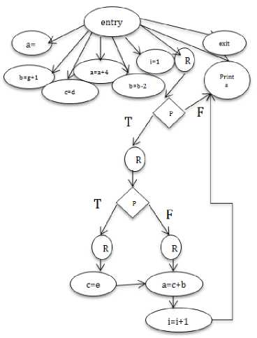
Fig.2. Construction of CDG

• C.    Construction of DDG

DDG is Data Dependence Graph, which depicts the data dependences between segments of a program. If there is a data dependency [12] from a block ‘X’ to block ‘Y’, then the segment represented by ‘X’ assigns some value to a variable, which will be used at the segment represented by ‘Y’. Here we have chosen a reachability algorithm to identify data dependences between statements or modules. Preferably we have selected blocks [18] due to clumsiness created due to individual statements consideration. For every block we have created four sets of values [8], GEN[B] is set of variables their values are currently used in block B, prior to any definition of that variables. KILL[B] is set of variables assigns some values in B, prior to any use of that variable in B. OUT[B] is set of variable active after that block B or OUT[B]= IN[S], where S is a successor of B. IN[B] is set of variable active at the beginning of that block B. IN[B]=GEN[B] (OUT[B]-KILL[B]). The DEF,KILL,IN and OUT are to be calculated for every statement in the program and OUT set has to be computed for predicate or region nodes in CDG.

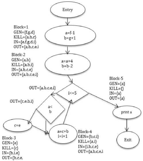
Fig.3. Construction of DDG

In our example, GEN of first block is f, g and d, because f, g and d are used on the right hand side of the three assignment statements before they are assigned any values. In fact, they are not assigned any values at all. Whereas, in the case of second block, a and b are used; before they are assigned a values. So, GEN will be a and b and KILL set do not contain a, b because of their accessibility before an assignment, but while exiting this block a and b assigned new values which are not used in that block i.e., KILL set also contains a and b. Even in case of simple assignment statement this is true, i.e., e is generated where as c is killed. As discussed earlier for predicate nodes only OUT sets will be calculated, for the first predicate node (i<=5) the OUT set contains a,b,c,e, and i because these variables are active or used in the processing after this block. For every predicate node there are two outgoing lines one for true and other for false. In Block-3, variable ‘e’ is used at right hand side, so it is included in GEN set and KILL set contains ‘c’; it is assigned a value, which is never used in this block. IN sets are calculated by using above said formulae or we can consider only those variables which are active at the beginning of the block. In Block-4, GEN set contains b,c, and i because their values are used in right hand side of a statement where as KILL set contains a and i because these values are not used in the same block. OUT and IN sets are calculated by using same process described in previous step. Finally in last block, only print statement is there, GEN set contains only a and KILL set contains no value because no assignment statements in this block and IN and OUT is same, which contains only a.

After combining above two modules, we have constructed PDG in Fig.4. For predicate nodes we have used diamond symbol and rest of all other purposes oval shape symbol has been used.

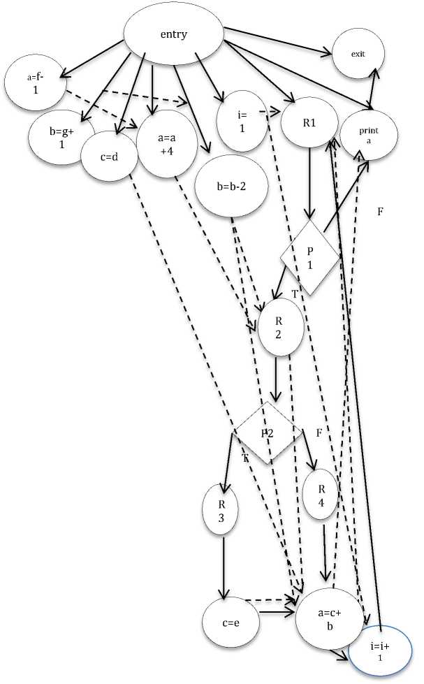
Fig.4. Construction of PDG

• ->   Data dependence lines

• ■^    Control dependence lines

• III.    Identification of Parallel Modules

In our approach, call Reachability Definitions to construct GEN, KILL, IN and OUT sets, then we consider all the vertices in a topological sequence. For every vertex ‘v’, find out the nearest predecessor ‘u’, if intersection of KILL[u] and IN[v] has some entries i.e., they have dependencies, then v and u can not be executed parallel. Otherwise they can be executed parallel. Demonstrated through an example in fig. 5.

Algorithm Parallel_Modules_Identification() {

Call Reachability Definitions (G)

Call Topological Sort (G)

For all vertices vε V(G) in topological order do {

Find vertex u ε nearest predecessor of v p = KILL [u] ∩ IN[v]

If (p!=  )

{

Sequential execution required

} else { Independent modules Parallel execution }

} }

• A.    Reachability Definitions

In Graphical representation of data, reachability [20] means path existence between any two vertices of a graph. In our approach discussing about reachability of definitions of a variable means the values assigned to a variable in a particular block is approachable to any other block, i.e., is used by any other variable in other block or vertex. We began with finding out GEN and KILL sets construction, then initialized IN sets of all the vertices to GEN set of that node. We have considered a change variable as flag, if it doesn’t change it’s value that means final sets for IN and OUT is ready. Till then update IN and OUT sets as mentioned in the algorithm.

Algorithm Reachability Definitions (G) {

GEN[B]= set of variables used in block B;

KILL[B]=set of variables has definitions in block B; for all blocks in a program do

{

IN[B]=GEN[B]

} change=0;

do

{ for each block B do

{ if ( block is a predicate node || region node) then OUT[B]=      OUT[P], where P is a predecessor of B else { // forward flow

IN[B]=       OUT[P], where P is a predecessor of B

OUT[B]=(OUT[B]-KILL[B])      GEN[B];

change=1;

// backward flow

OUT[B]=       IN[S],where S is a successor of B

IN[B]=GEN[B]      (OUT[B]-KILL[B])

change=1;

} while(change);

}

• B.    Topological Sort

A topological sort of a given graph G=(V, E) is “ A linear Ordering of vertices [16] such that if there is an edge from u->v then ‘u’ precedes ‘v’ in the sequence”. Many algorithms developed [10] to get topological sequence of a graph. The primary applications or Real word applications are instruction scheduling, ordering of formula cell evaluation when re-computing formula values in spreadsheets, logic synthesis, determining the order of compilation tasks to perform in make files, data serialization, and resolving symbol dependencies in linkers. It is also used to decide in which order to load tables with foreign keys in databases.

Algorithm Topological Sort (G) {

Call DFS (G);

Insert nodes traversed through DFS in the descending sequence of finishing times in to a linked list;

Return list of nodes of a linked list;

}

Global declaration of t=0;

Algorithm DFS (G) { for each vertex v ∈ V(G) do visit[v]=false; //visit[] is a Boolean field if a vertex visited, then it is true otherwise it is false for each vertex v ∈ V(G) do if(visit[v]==false) then call DFS_VISIT(v);

}

Algorithm DFS_VISIT(v) { t++;

visit[v]=true;

S[v]=t;           // starting times

For each vertex u ∈ adj(v) do

If (visit [u]==false)

{

Call DFS_VISIT (u);

} t++;

F[v]=t;           //finishing times

}

• IV.    Performance Analysis

Performance of a proposed approach can be demonstrated: Reachability algorithm takes O (n2) time, where ‘n’ is number of statements in a program, and number of statements is equal to number of vertices in a graph, i.e., time complexity can be expressed as O (V2). Topological sort [17] requires O (V+E) time and by considering the vertices in topological sequence, finding out independent modules requires O (V2) time. Total time complexity of our approach is:

I T(n)   = O(V²)+ O(V+E)+ O(V²)

= 2*O(V²)+ O(V+E) if a graph is sparse

= O(V2 '                 ■

• A.    Sequential versus Parallel execution

If a single processor is used for the execution of below program segment, first block requires exactly m*n time, where as second block requires s*e time and the last block requires o*p time. The total time required is (Linear time complexity)

T (n)= θ (mn+op+se)

for i= 1 to m do { for j=1 to n do {x++ y—}}

GEN={m,n,i,j,x,y}

KILL={x,y,i,j}

IN={m,n,i,j,x,y,k,l,o,p,a,b,c,s,e }

OUT={k,l,o,p,a,b,q,c,s,e,x,y,i,j

GEN={q,c,s,e,x,y}

KILL={q,c,x,y}

IN={ q,c,s,e,x,y }

OUT={k,l,o,p,a,b,x,y,q,c} for q=1 to s do { for c= 1 to e do {x++ y++ }}

GEN={o,p,k,l,a,b} KILL={a,b,k,l} IN={ o,p,k,l,a,b} OUT={o,p,k,l,a,b}

for k= 1 to o do { for l=1 to p do {a++ b=*b }}

Fig.5. Construction of GEN,KILL,IN,OUT sets

By taking sample data a graph has been plotted with red colored line. For thinking in parallel perspective, find out all four sets for individual modules, i.e., GEN, KILL,

IN and OUT. Make the comparison between IN set data with KILL set of near by predecessor to determine independence modules. If we use two processors for the execution of the same code, it required s*e*f time due to parallel execution of these three independent modules. A graph has been plotted below with blue colored line.

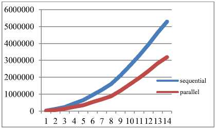
Fig.6. Performance Analysis

• B.    Speedup

In parallel computing, the speedup is nothing but ratio between sequential and parallel execution times i.e., it reflects what extent a parallel algorithm is faster than a corresponding sequential algorithm. Speedup is a factor, which improves performance in terms execution after enhancement of resources. In Table 1, observe the data in the column speedup, it varies from 1.5 to 2.0 i.e., The parallel approach is 1.5 to 2 times faster than sequential approach, which has been illustrated through a pictorial representation or in the form of a graph in below figure.

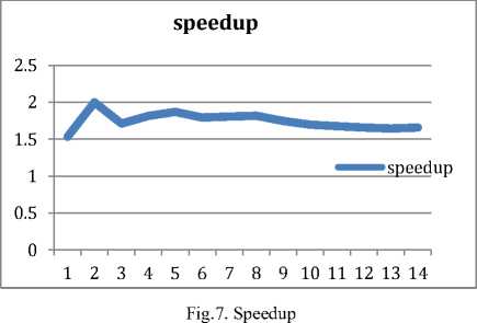
In Table 1 data is considered randomly to determine caliber or performance of a suggested system.

Table 1. Comparison of sequential and Parallel Execution time

m	n	s	E	O	p	m*n	s*e	o*p	Sequential	Parallel	Speedup
100	50	50	200	400	20	5000	10000	8000	23000	15000	1.533
200	100	100	400	600	100	20000	40000	60000	120000	60000	2
300	150	200	450	800	120	45000	90000	96000	231000	135000	1.71
400	200	300	550	1000	200	80000	165000	200000	445000	245000	1.81
500	250	400	550	1200	250	125000	220000	300000	645000	345000	1.86
600	300	500	700	1400	300	180000	350000	420000	950000	530000	1.79
700	350	600	750	1600	350	245000	450000	560000	1255000	695000	1.80
800	400	700	800	1800	400	320000	560000	720000	1600000	880000	1.81
900	450	800	1000	2000	450	405000	800000	900000	2105000	1205000	1.74
1000	500	900	1200	2200	500	500000	1080000	1100000	2680000	1580000	1.69
1100	550	1000	1350	2400	550	605000	1350000	1320000	3275000	1955000	1.67
1200	600	1100	1500	2600	600	720000	1650000	1560000	3930000	2370000	1.65
1300	650	1200	1650	2800	650	845000	1980000	1820000	4645000	2825000	1.64
1400	700	1300	1700	3000	700	980000	2210000	2100000	5290000	3190000	1.65

• V.    Conclusion

This paper presents a research plan with an overarching goal to ensure that effectiveness of an approach in identifying parallel segments. While this framework provides new scenario to identify parallel modules. A given application is represented using AST and further it is converted into PDG, and by using reachability definition concept we identified concurrent modules.

• VI.    Future Work

After identifying parallel modules according to our approach, this research plan can be extended for the execution of those modules on heterogeneous parallel architectures according to the topology suggested. This work can further bring in to the parallelization scenario.