Performance Analysis of Classification Methods and Alternative Linear Programming Integrated with Fuzzy Delphi Feature Selection

Published Online September 2013 in MECS DOI: 10.5815/ijitcs.2013.10.02

• I.    Introduction

  The applications of classification methods are wide-ranging and the advent of powerful information systems since the mid-1980s has renewed interest about classification techniques [1]. Differentiating between patients with strong prospects for recovery and those highly at risk, between customers with good credit risks and poor ones, or between promising new firms and those likely to fail, are among the most known applications [2]. Especially managers use classification techniques to make decisions in different business operation areas. At its broadest, classification could cover any context in which some decision is made on the basis of currently available information. Then,

classification is a method for making judgments in new situations [3]. For instance, rather than targeting all customers equally or providing the same incentive offers to all customers, managers can select those customers who meet some profitability criteria based on purchasing behaviors [4]. However, due to the nature of classification problem, a spectrum of techniques is needed because no single technique always outperforms others under all situations [5]. Various methods have been proposed for solving classification problems which can be divided into two categories: parametric and non-parametric discriminant methods. There are no pre-defined assumptions in non-parametric methods. However, parametric methods make strong parametric assumptions such as multivariate normal populations with the same variance/covariance structure, absence of multi co-linearity, and absence of specification errors [6]. Classification methods can also be grouped as statistical approaches such as Linear Discriminant Analysis (LDA) and Logistic Regression (LR), artificial intelligence or machine learning techniques such as Artificial Neural Network (ANN) and Support Vector Machine (SVM) and Operation Research techniques such as Linear Programming (LP) and Goal Programming (GP).

The earliest discriminant method proposed by Fisher in 1936. This method of discrimination requires that the sample to be distributed normally and the variancecovariance matrices of the two groups to be homogeneous. Mangasarian also was the first who used LP method for classification problems [7]. Linear Programming method have some advantages over other approaches which can be enumerated as follow: First, there is no assumption about the functional form and hence it is distribution free. Second, they are less sensitive to outliers. Third, they do not need large datasets. Nonetheless, linear programming methods also have a disadvantage, which is the lengthy computation. However, immense increase in computing power and drop in computing cost overcome the disadvantage and made LP methods practical.

This research uses Linear Discriminant Analysis, Logistic Regression, Support Vector Machine, and Artificial Neural Network vis-a-vis Multi-Group Discriminant Linear Programming (MDLP) discriminant analysis to classify the customers of an Internet Service Provider company based on their real demographic data including age, gender, education, income, purpose, in order to present the strength and accuracy of classification models, especially for MDLP.

One major problem of classification methods, especially for small businesses or E-businesses, is the dispersed, deficient and redundant data in their databases. For this reason, researchers usually use synthetic or simulated data; however, it is not realistic. That is why the application of fuzzy Delphi is suggested in this study for the selection of the required features. This helps companies to classify their customers with their current rudimentary databases; otherwise they should wait for months or years for depositing the data and it is obviously undesirable in today competitive environment.

To achieve this purpose, the ISP company dataset was used to segment the customers based on RFM (Recency, Frequency and Monetary) model by different clustering methods such as K-means, Self-OrganizingMap, Two-Step Clustering and Data Envelopment Analysis. The customers have been grouped in three distinct segments. Each segment comprises its own average R, F and M value which is an indication of customer lifetime value (CLV). The acquired information obtained in clustering step, is utilized for the purposes of this paper.

The organization of this paper is as follows: brief description of various classification methods which will be covered in section 2. Section 3 presents data preparation using fuzzy Delphi. Section 4 shows the computational results and exhibits the performance of different classification methods including MDLP.

• II.    Classification Methods

• 2.1    Logistic Regression (LR)

Well-known classification methods including Logistic Regression, Linear Discriminant Analysis, Artificial Neural Network, Support Vector Machine and Multi-group Discriminant Linear Programming are introduced in this section briefly.

Logistic regression is a modeling procedure where a set of independent variables are used to model a dichotomous criterion variable using maximum likelihood estimation (MLE) procedure. Therefore, it is appropriate for direct marketers who would like to model a dichotomous variable such as buy/don’t buy, default/don’t default, and so on. The availability of sophisticated statistical software and high speed computers has further increased the utility of logistic regression. The predicted value is the response probability, which varies from zero to one [8]. In logistic regression, the probability of a dichotomous outcome is related to a set of predictor variables in the form of following function:

In I -p 1 = p x = P o + P 1 x + P 2 x 2 + ... + P n X n    (1)

• 1 ¹ - P )

• 2.2    Fisher Linear discriminant Function (LDF)

• 2.3    Artificial Neural Networks (ANN)

• 2.4    Support Vector Machine

• 2.5 Multi-Group Linear Programming

  Linear Programming (LP) or at its broadest Mathematical Programming (MP) approaches are nonparametric and have attracted interests of many researchers, because these methods do not make strict assumptions about the data analyzed, are less influenced by outlier observations and are flexible in incorporating restrictions. The publication of the original LP models for two-class classification by Freed and Glover inspired a series of studies [16]. Some of these studies reported pathologies of the earlier MP models, some provided diagnoses, and others offered remedies [17]. The method uses a weighting outline to establish a critical value or cutoff point that serve as a breakpoint between two successful and unsuccessful groups. Afterwards, Freed and Glover proposed a set of interrelated goal programming formulations. They proved the potential of these formulations with the help of a simple example of assigning credit applicants to risk classifications. However, for decades, MP approaches have been limited to two-class methods because of the lack of powerful and simple models. Among the various MP models for classification problem, the model proposed by Lam and Moy (1996) have recently attracted the interest of researchers [17]. They modified the earlier model proposed by Freed and Glover [16] for multi-group classification problem and proved that it is more powerful in terms of hit-rate criterion and its stability than statistical methods. Their model is as follows:

Where p is the probability of the outcome of interest, в is the intercept term, and P i (i=1,...,n) represents the coefficient associated with the corresponding explanatory variable x i (i=1,...,n) [9]. The dependent variable is the logarithm of the odds , [ log [p /(1-p)]] which is the logarithm of the ratio of two probabilities of the outcome of interest. For instance, if we are interested to measure the effect of independent variables such as consumption of tobacco cigarette and alcohol on blood status indices and 25 of 100 persons have indications in their blood, then it can be said the odds is 25 to 75 or one-third. However, when the probability of occurrence is too high or too low, odds go to infinity. Then the logarithm of odds is usually used to resolve this problem. The logarithm of odds is named logit . If the logit is negative, it means the odds is against the event occurrence and vice versa. If the odds is 50-50, the logit is zero. In this research, we use multinomial logistic regression, because the dependent variable is a three-class categorical variable which indicates three pre-defined market segments.

Database marketers frequently use discriminant analysis as an alternative to logistic regression. Discriminant analysis is a multivariate technique identifying variables that explain the differences among several groups and that classify new observations or customers into the previously defined groups [10]. This method separates classes by linear frontiers to group the data to be classified around the centre of gravity (average) of each class and to create a linear hyperplane between the classes. This method requires certain assumptions: the normality distribution of the samples, homogeneity of the variances-covariances matrices [2]. If we have n variables, the discriminant function is as follows:

Z i =b 0 +b 1 ^X 1 i +b 2 ^X2i⁺ ^ ^+bn X ni                     ⁽²⁾

Where Xij is ith individual’s value of the jth independent variable, bj is discriminant coefficient for the jth variable, Zi is ith individual’s discriminant score and Zc is critical value for the discriminant score. If Zi>Zc, then individual i belongs to class 1, otherwise to class 2. If there are two classes, the separating boundary is a straight line. Generally, the classification boundary is an (n-1) dimensional hyperplane in n space [11]. LDF depends on parameters b0, b1,...,bn and an algorithm of training is used to determine these parameters. This algorithm aims to satisfy the criterion associated with the model which generally aims to minimize the error of classification.

The foundations of Support Vector Machines (SVM) have been developed by Vapnik and gained popularity due to many promising features such as adequate empirical performance [13]. The goal of support vector machine is to find the particular hyperplane (called the optimal hyperplane) which maximally separates two classes [14]. The observations that are closest to the optimal hyperplane are called support vectors Xs. The optimal weighting vector can be derived by solving a quadratic optimization problem. Support vectors can be derived once the optimal weighting vector is determined. These vectors play a critical role in support vector machines. Since support vectors lie closest to the decision surface, they are the most difficult observation to classify. However, only these closest instances are required to classify new instances so that the rest of the instances play no role in predicting the class of new ones. It means that a set of support vectors uniquely defines the optimal hyperplane. However, the biggest disadvantage of the linear hyperplane is that it can only represent linear boundaries between classes [15]. One way of overcoming this restriction is to transform the instance space into a new “feature” space using a nonlinear mapping. A straight line in feature space does not look straight in the original instance space. That is, a linear model constructed in feature space can represent a nonlinear boundary in the original space. Briefly speaking, the idea of support vector machines is based on two mathematical operations: (1) nonlinear mapping of the original instance space into a high dimensional feature space, and (2) construction of an optimal hyperplane to separate the classes. In other words, we need to derive the optimal hyperplane defined as a linear function of vectors drawn from the feature space rather than the original instance space [10]

Suppose there are totally n observations distributed in m groups so that n=n 1 +n 2 + ...+n_m in which n k is the number of observations in group k , (G k .). If x ij is value of the j-th variable (attribute) for the i-th observation in the sample and we consider q variables, for each pair of groups ( u, v, u= 1 ,...,m- 1 and v=u+ 1 ,...,m ), the minimization of the sum of deviations model is as follows:

n

min ∑ d i∈Gu∪ Gv

St :

∑q wj(xij -xj(u))+di ≥0,  ∀i∈Gu j=1

∑q wj(xij -xj(v))-di ≤0,  ∀i∈Gv j=1

∑q wj(xj(u) -xj(k)) ≥1, j=1

d≥0

variable j and x ( k ) is the mean of the j-th variable in group k ( k=1, 2,..., m ) which defines as follows:

xj(k)=∑i∈Gxij /nk                         (4)

The objective function minimizes the sum of all the deviations. The first two constraints force the classification scores of the observations in G_k to be as close to the mean classification score of group k as possible by minimizing d_i and the last constraint is a normalization constraint in order to prevent trivial values for discriminant weights.

Now the calculated w j values are used to obtain the values of classification scores in each group G k :

q

S _i = ∑ w _j x _ij , for i ∈ G _k                         (5)

j = 1

Then the cut-off scores ( C_uv ), which indicate the separating boundary between the groups, are calculated by the following LP model:

in which, di is the deviation of the individual observations from cut-off scores (c), wj is the weight of m-1 m

min∑ ∑ (∑diuv +∑diuv)

u = 1 v = u + 1 i ∈ G_ui ∈ G_v

^{St :}                                                                                               (6)

Siuv + diuv ≥ Cuv,for u =1,...,m-1,v=u+1,...,m,  i∈ GuSiuv - diuv ≤ Cuv,for u =1,...,m-1,v=u+1,...,m,  i∈ Gv in which, Cuv are unrestricted in sign. This process converts the classification problem to m(m-1)/2 distinct two-group problems which is solved separately.

Another extension of this model is offered by Pai et al [1] based on the model of Lam and Moy [18] in which, the mean is substituted by median. They proved this substitution increases the efficiency of the model in respect of hit rate especially when the distribution of data set is abnormal or skewed. Therefore, this study uses the median instead of mean in (4).

• III.    Data Preparation

  To show the efficiency of aforementioned classification models in real settings, we use a dataset related to 6000 customers provided by Irangate Internet Service Provider (ISP) Company for a five years period from 2007 to 2012. Irangate is a major ISP company in Iran whose mission is to satisfy customers' needs for different kinds of internet services such as E-commerce

and DSL. This Company offers its customers different packages of bandwidth, time and charges of internet services.

The required data for classification purposes which is scattered within databases of different company departments should be gathered, combined, refined and prepared. After removing redundant and inconsistent data, 5271 records remained. Recency, Frequency and Monetary (RFM) model is applied to segment the customers using clustering ensemble method in which K-means, Self-Organizing Map (SOM) and Two-Step clustering are used. Cluster ensembles can be formed in a number of different ways such as the use of a number of different clustering techniques, the use of a single technique many times with different initial conditions and the use of different partial subsets of features or patterns [19]. The K-means algorithm for partitioning is base on the mean value of the objects in the cluster and the term K-means was suggested by MacQueen [20] for describing an algorithm that assigns each item to the cluster with the nearest centroid or mean. The SOM is an unsupervised neural network learning algorithm and forms a mapping the high-dimensional data to twodimensional space and forms clusters to represent groups of nodes with similar properties [21]. In two-step clustering, in the first step, cases are assigned to pre-clusters and in the second step; the pre-clusters are clustered using the hierarchical clustering algorithm.

Based on the clustering ensemble concept and using the aforementioned clustering techniques, three customer segments identified with different internet usage pattern based on RFM model which is shown in Table 1. RFM is a useful marketing technique to improve customer segmentation. It is used for analyzing customer behavior such as how recently a customer has purchased (recency), how often the customer purchases (frequency), and how much the customer spends (monetary) [22].

Table 1: Three customer segments identified based on RFM model

	Number Of Customer	Recency Score Mean (Month)	Frequency Score Mean (Times)	Monetary Score Mean (Giga Byte)
Cluster 1	2387	4.838	2.062	2.582
Cluster 2	1776	6.808	7.068	6.306
Cluster 3	1108	2.407	1.977	7.836

According to Table 1, the average recency, frequency and monetary of the segments are totally different. As it is shown, cluster 2 is the segment of high-valued customers, because the average recency, frequency and monetary of this segment is the highest. Cluster 3 also needs more concern and attention. While these customers have higher monetary in comparison to two other segments, they have less purchase frequency and recency scores. This segment includes customers who are leaving the company. The customer churn should be noticed by the managers.

However, when it came to classification process, it is found that the company dataset of this small E-business lacks some required data such as customer profile data. Concerning the data, the company was not well-organized due to the lack of long-term business strategy and required knowledge and experiences. Therefore, Fuzzy Delphi approach has been employed to find the most important customer features we could use as predictors in classification models.

• IV.    Fuzzy Delphi Application

As it is pointed out, it is possible to have a deficient database which does not allow to goes through classification process. This study proposes to use fuzzy Delphi method to encounter the problem and gather the required data. Fuzzy Delphi method was proposed by Ishikawa et al. and it was derived from the traditional Delphi technique and fuzzy set theory [23]. The traditional Delphi method is a structured communication technique, originally developed as a systematic, interactive forecasting method in which several rounds of anonymous written questionnaire surveys conducted to ask for experts’ opinion [24]. Noorderhaben [25] indicated that applying the Fuzzy Delphi Method to group decision can solve the fuzziness of common understanding of expert opinions. Previous researches have applied triangular fuzzy number, trapezoidal fuzzy number and Gaussian fuzzy number for fuzzy membership functions. This study uses triangular membership function denoted by (m, α, β) in which the point m, with membership grade of 1, is called the mean value and α, β are the left hand and right hand spreads of m respectively.

To utilize the fuzzy Delphi method following steps were taken:

• 1-    The relevant literature was studied to compile a list of variables and eventually eight variables as age, gender, education, income, purpose, lifestyle, occupation and location were derived.

• 2-    Ten experts from different departments of company were invited and a questionnaire survey in the form of table 2 was carried out. They were asked to determine the importance of each variable in identifying the customers for classification purpose as very high, high, moderate, low, very low. Table 2 is also shows the results. For instance, five experts evaluate the education as very high, four people evaluate it as high and one people evaluate it as moderate.

• 3-    To change the experts’ opinion to triangular membership function, the linguistic variable scale (Fig.1) and its equivalent triangular numbers (Table 3) were used. If the expert’s opinion i for variable A is shown by

5 . = 1        5 i = 1       5 i = 1

A i = ( m i ^{, a} i , ^e

The fuzzy average of s experts opinions for that variable is obtained by sss

Aave = (1 Z m.-УаД Z P)

в

X = m + —

• 4-    In order to rank the variables, the average of experts’ opinion is calculated by Minkowski formula (9). The fuzzy results are shown in Table 4. According to Table 4, the most important variables, education, purpose, income, gender and age, are used as predictors.

- а

⁴                                    (9)

Then by interviewing customers of each segment through the phone, the required information about their age, gender, educational level, annual income and main purpose of internet usage have been acquired. A total of 1808 customers were interviewed. These variables have been quantified by encoding them which is shown in Table 5. Considering these data along with age and income, there will be 13 variables as input for classification routine.

Table 3: Triangular fuzzy numbers and its equivalent linguistic variables (Mirsepasi et al, 2010)

Triangular Fuzzy Numbers and its Equivalent Linguistic Variables
Linguistic Variable	Triangular number (m, a, p)
Very High	(1.00 ,0.25, 0.00)
High	(0.75,  .15, 0.15)
Moderate	(0.50, 0.25, 0.25)
Low	(0.25, 0.15, 0.15)
Very Low	(0.00, 0.00, 0.25)

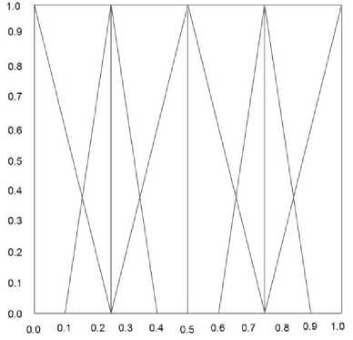
Fig. 1: Linguistic variable scale

In next sections, the classification process is made using this information and based on the aforementioned models.

V. Performance Evaluation

The performance of classification models can be measured by several criteria such as accuracy, hit rate, confusion matrix and etc. Accuracy refers to the percentage of correct predictions made by the classification model when compared with the actual classifications in the validation data. A hit rate is the ratio of the number of correctly classified targets to the number of classified targets. A confusion matrix displays the number of correct and incorrect predictions made by the classification model compared with the

Table 2: Experts’ opinion about importance of variables in classification of customers

Variable		Agreement
		Very High	High	Mod	Low	Very Low
1	Location	0	0	2	5	3
2	Life Style	0	0	2	4	4
3	Education	5	4	1	0	0
4	Income	2	4	2	1	1
5	Purpose	5	2	2	1	0
6	Age	1	2	1	3	3
7	Gender	0	2	3	3	2
8	Occupation	0	1	2	4	3

Table 4: Variable selection by fuzzy Delphi

Features		Triangular Fuzzy Average ( m , a , P)			De-fuzzy Average
1	Age	0.375	0.150	0.200	0.387
2	Gender	0.625	0.200	0.150	0.612
3	Education	0.850	0.210	0.085	0.819
4	Income	0.625	0.175	0.150	0.619
5	Purpose	0.775	0.220	0.095	0.744
6	Location	0.175	0.105	0.180	0.194
7	Life Style	0.100	0.06	0.200	0.135
8	Occupation	0.275	0.125	0.125	0.275

Table 5: Different levels of categorical variables

Variable Code Gender Female=0, Mail=1, Education Below Diploma=0, Diploma=1, University Diploma=2, B.S.=3, M.S.=4, PHD=5 Purpose Research=1, Business=2, Social Networking=3 actual classifications in the validation data. The matrix is n-by-n, where n is the number of classes. In order to use the different criteria, typically hold-out method is used in which the dataset is partitioned into two portions: training data and evaluation data. In other words, a percentage of the records are used to build the classification model and the remaining records are used to validate the model. In this study, for all the methods of classification, data records related to 1808 customers are divided using holdout sampling method into training and validation data sets with the ratio of 65 and 35 percent, respectively. Then, the accuracy of classification models are obtained in Clementine and Matlab environment software and compare with each other.

• 5.1    The results of LDF

As it is mentioned earlier, in order to use this method some criteria should be met such as normality of the sample distribution. Shapiro Wilks test proved that except age, remaining variables are not normal. However, to get an insight of the Fisher discriminant analysis, we ignore these assumptions. The aim of linear discriminant is to select the most significant variables and to determine the Fisher’s linear discriminant function. Table 6 illustrates the most significant variables using the Lambda of Wilks (LW). LW is used in discriminant analysis such that the smaller the lambda for an independent variable, the more that variable contributes to the discriminant function. LW varies from 0 to 1, with 0 meaning group means differ, and 1 meaning all group means are the same [26].

Table 7 shows that the most significant variables in differentiating the three customer segments in terms of Wilks’ Lambda are income and purpose. To find the Fisher’s linear discriminant functions which shown in (2), the coefficients of these two variables and the constant term should be determined.

Table 6: The discriminant power of variables

Vatiable	Wilks' Lambda
Age	.968
Sex	.999
Education	.979
Purpose	.951
Income	.866

Table 7: The coefficients of LDF method

	Segments
	1	2	3
Purpose	3.374	2.862	3.531
Income	.074	.091	.132
(Constant)	-5.506	-4.803	-7.319

Therefore, we have three discriminant functions which each of them discriminate one customer segment from others as follows, according to (2):

F 1 = -5.506 + 0.074 × income + 3.374 × purpose

F 2 =-4.803 + 0.091 × income + 2.862 × purpose

F 3 =-7.319 + 0.132 × income + 3.531 × purpose

To show the validity of the equations, the correct classifications for validation data set are calculated. Table 8 exhibits the number and percentages of records classified correctly.

True classifications into the first, second and third segments are respectively 52.2, 50.8, and 46 percent which yields 49.7 percent, in average. The results show that Fisher discriminant analysis performance is not adequate concerning correct classification criterion. It is because the model pre-assumptions are not verified

Table 8: Correct classifications of LDF method

Classification Results
	Class	Predicted Group Membership			Total
Count		1	2	3
	1	206	145	44	395
	2	99	199	94	392
	3	113	89	172	374
%	1	52.2	36.7	11.1	100.0
	2	25.3	50.8	24.0	100.0
	3	30.2	23.8	46.0	100.0

• 5.2    The results of Logistic Regression (LR)

20.26 × [Purpose=0] + 0.9714 × [Purpose=1] + 0.7218 × [Purpose=2] + 0.0562 × Income - 0.8118

• 5.3    The results of Artificial Neural Network(ANN)

The logistic regression is a method that doesn’t require any assumption. Therefore, it can be used in situations that the assumptions of linear discriminant procedure are not verified. To evaluate the LR model, discriminant functions are derived by training data and new observations will classify by the functions. If the segment one is considered as reference group according to (1), logistic regression finds two discriminant equations for segments two and three as follows:

F 3 = -4.096 + 0.4978 × [Sex=0] - 0.5183 × [Education=0] + 1.695 × [Education=1] + 1.972 × [Education=2] + 1.753 × [Education=3] + 1.54 × [Education=4] - 20.76 × [Purpose=0] - 0.2584 × [Purpose=1] - 0.1181 × [Purpose=2] + 0.1047 × Income

F 2 = 0.0879 × [Sex=0] - 2.836 × [Education=0] -0.4651 × [Education=1] - 0.9607 × [Education=2] -0.8236 × [Education=3] - 0.981 × [Education=4] -

Table 9: Correct classification of LR method

Classification
Observed	Predicted
	1	2	3	Percent Correct
1	231	121	43	58.5%
2	102	196	94	50.0%
3	113	72	189	50.5%
Overall Percentage	38.4%	33.5%	28.1%	53.1%

Classification of new observations and calculation of correct classification can be done based on these equations, as shown in table 9. The overall percentage of correct classification is 53.1%. Although it is a better value than of Fisher linear discriminant, it is still low.

Different ANN methods use distinctive architectures or topologies including several hidden layers and various neurons in each hidden layer. To show the performance of artificial neural network, the aforementioned topologies which consider different structures in employing training data are used. Table 10 indicates the performances of these methods along with their structures. As it is shown, exhaustive prune method with the most complicated structure yields a better performance than of the other methods. Table 11 indicates the performances of ANN for both training and validation data set. The average correct classification of different structures is 58% and 60% for training and validation datasets, respectively.

Table 10: Different ANN performance and structure

Function	Input Layer Neurons	First Hidden Layer Neurons	Second Hidden Layer Neurons	Third Hidden Layer Neurons	Output Layer Neurons	Correct Classification (%)
RBFN	13	20	-	-	3	46.8
Dynamic	13	8	6	-	3	52.6
Exhaustive Prune	13	26	16	-	3	70.6
Multiple	13	12	12	11	3	64.4

Table 11: ANN functions performance for training and testing data

Method	Training		Validation
RBFN	526	45%	308	48%
Exhaustive Prune	848	73%	481	74%
Dynamic	618	53%	354	55%
Multiple	725	62%	409	63%
Average	679	58%	388	60%

• 5.4    Support Vector Machine (SVM)

• 5.5    Multi-Group Linear Programming

• 5.5.1    Training Process:

SVM uses mathematical kernel functions to map the data into a high-dimensional feature space in order to categorize the dataset even when the data are not linearly separable. RBF, polynomial, sigmoid and linear kernel functions are used to classify the dataset and evaluate correct classification for training and validation data. The results are shown in table 12.

Table 12: SVM’s correct classification for training and validation datasets

Function	Training		Validation
	Count	Percent	Count	Percent
RBF	675	58%	363	56%
Polynomial	841	72%	413	64%
Sigmoid	442	38%	239	37%
Linear	595	51%	353	54%
Average	638	55%	342	53%

Although polynomial function yields a better performance, however the average correct classification is 55% and 53% for training and validation dataset respectively. In addition, the correct classifications of polynomial function for training and validation data sets are 72% and 64% respectively. This shows a large difference and it is an indication of model instability.

Based on the multi-group linear programming approach which introduced in section 2.5 and utilizing the formulations 3-6, the performance of MLP model in classification is evaluated. For this purpose, a Matlab program is prepared. The same hold-out sampling method with 65-35 percent for training and validation process is used.

Table 13: The weights of customer features in paired groups

Segments 1 and 2
W 1	W 2	W 3	W 4	W 5
0.025721	0.093712	-0.11725	0.478386	-0.13682
Segments 1 and 3
W 1	W 2	W 3	W 4	W 5
0.004049	0.086293	-0.01683	-0.12602	-0.062
Segments 2 and 3
W 1	W 2	W 3	W 4	W 5
0.016368	0.012801	0.262658	-0.66177	-0.06957

Now the cut-off scores which indicate the separating boundary between each pair of groups are obtained by Model 6. Table 14 shows the results.

Table 14: Cut off scores

	Cluster 1	Cluster 2	Cluster 3
Cluster 1		-0.9893	-1.32734
Cluster2			-1.89657
Cluster 3

As it was mentioned in section 2.5, the deviations of individual objects (di) are minimized by MDLP formulation. Therefore, having the weights of variables and cut-off scores and using (5), classification scores of training dataset is obtainable. Then, the corresponding class for each customer is predicted. Table 15 exhibits a small portion of the results. As it is shown, except customers 6 and 14 which belong to segment 1 but has been assigned to wrong groups, the other customers are assigned correctly. The percentage of correct classification for paired groups is shown in table 16. This table shows that correct classification between cluster 1 and 3 is the highest and the average is 66%. This performance is near the best results of unique structures of artificial neural network.

• 5.5.2    Validation

Now using cut-off and weight scores obtained in the previous stage, the classification score of validation dataset is obtained. Table 17 shows the result. The table indicates that the correct classification for validation data is slightly better than correct classification for training data. However, the average correct classification is 69% and it is very near to the average correct classification for training data which shows model stability

Table 16: The correct classification percentages of MDLP method for training data

Cluster Comparison	Correct Classification
1 & 2	65%
1 & 3	69%
2 & 3	63%
Average	66%

Table 17: The correct classification of MLP method for testing data

Cluster Comparison	Correct Classification
1 & 2	68%
1 & 3	73%
2 & 3	65%
Average	69%

Table 18: Comparison of performance of different classification methods

Model	Training	Testing
ANN	58%	60%
LDF	50%	53%
LR	53%	55%
SVM	55%	53%
MLP	66%	69%

• VI.    Comparison of the Performance of the Models

This section compares the performance of aforementioned classification models. Table 18 includes the average correct classification of the models for training and validation datasets. As it is shown, the average correct classification of multigroup linear programming is considerably higher than other models.

However, a major concern for application of multigroup linear programming is its requirement of relatively high amount of running time. Using an Intel Pentium Dual CPU and E2200 @ 2.2 GHz PC computer with 2G RAM,), it is slightly slower than the other models and takes 3 minutes and 40 seconds to run the LP model for 1808 record datasets.

Table 15: Predicted and current customer class

Cluster 1 and 2				Cluster 1 and 3				Cluster 2 and 3
ID	Score	Predicted Class	Current Class	ID	Score	Predicted Class	Current Class.	ID	Score	Predicted Class	Current Class
3	-0.231	1	1	3	-0.888	1	1	601	-1.072	2	2
6	-2.552	2	1	6	-2.066	3	1	602	-2.036	3	2
7	-0.935	1	1	7	-0.754	1	1	604	-1.872	2	2
9	-0.342	1	1	9	-0.542	1	1	606	-0.491	2	2
12	-0.780	1	1	12	-1.219	1	1	607	-1.942	3	2
13	0.008	1	1	13	-1.213	1	1	610	-1.402	2	2
14	-1.029	2	1	14	-0.840	3	1	611	-3.916	3	2
15	-0.672	1	1	15	-1.517	1	1	613	-2.052	3	2
17	-0.989	1	1	17	-0.845	1	1	614	-2.477	3	2

This amount of time is comparable with the time required by other models.

the average performance of multi-group linear programming is considerably competent, at least for small and medium-sized data sets.

• VII.    Conclusion

Statistical and data mining classification methods have been used for years. Although different versions of mathematical programming for classification have introduced in the literature, but they have been ignored due to considerable running costs. However, the advent of powerful information system has resumed the application of mathematical programming due to its non-parametric nature which is not dependent of any assumptions. This study used well-known statistical and data mining methods vis-à-vis multi-group linear programming discriminant analysis in a real setting of a ISP company. The real life data often contaminated, because it is usually include noisy, incomplete and redundant data. Especially the problem of lack of required data is an important issue. To overcome this problem, we used fuzzy Delphi to extract necessitated data for classification purposes. The result proved that

Acknowledgments

The authors would like to thank the Irangate ISP Company, Isfahan, Iran, for providing the required data.