Performance Analysis of Deep Learning Techniques for Multi-Focus Image Fusion

The advancement of digital imaging has completely transformed the way we capture and interpret information. A fundamental property of digital photography is the depth-of-field (DOF) which pertains to the range of distances, in a scene that appears sharp and clear in an image. A camera’s DOF is strongly related to the quality of lens, sensor size and camera settings. It is desirable in many applications for the entire image to be sharp, but due to optical limitations, a traditional camera can only focus on a single plane resulting in objects outside this plane appearing blurry. This restriction in DOF can be problematic in fields where capturing details at distances is crucial such as surveillance and microscopy.

To address these restrictions, multi-focus image fusion (MFIF) has emerged as an essential approach to enhance the DOF in digital images. It is an important field of image processing and computer vision. MFIF combines information from multiple images, each with a varied focus depth, to create a single unified image in which all components are in focus. The objective of MFIF is to refine the visual clarity of images across the entire field of vision, irrespective of the restrictions imposed by conventional cameras. An example of MFIF is shown in Fig.1. Since the need for high-quality fused images continues to expand, professionals and researchers are continually looking for novel strategies and algorithms to help enhance the MFIF process. Such measures are critical for improving the ability of imaging process and opening latest possibilities in different fields. MFIF methods are widely classified into two types [2]: spatial domain-based methods and transform domain-based methods. These are traditional based approaches.

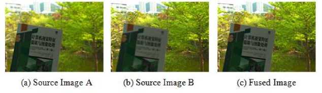
Fig.1. An illustration of MFIF using two source images. Image courtesy of [1].

Spatial domain-based approaches directly modify the pixel values in the images. The objective is to evaluate pixels from many input images and choose the more detailed one for the fused image. There are three categories of spatial domain based methods. These are pixel, region and block-based methods. Some commonly named are dense scale invariant feature transform (DSIFT) [3], quad-tree based methods [4], PCNN [5], guided filtering based methods (GFF) [6] among others. These approaches frequently employ sliding window method that evaluates the focus measure within small regions to determine which elements of each image are in focus [7–9].

Conversely, transform domain-based approaches firstly convert the images to a distinct realm, for instance wavelet or frequency domain, prior beginning the fusion process. The images are converted using mathematical techniques like Fourier Transform or the Wavelet Transform. The basic premise is that in the transform domain, it is simpler to distinguish between critical and less critical elements, such as edges and textures [8–10]. Following the transformation and selection steps, an inverse transform is employed to create a fused image in the spatial domain. These methods include Laplacian pyramid [11], dual-tree complex wavelet transform (DTCWT) [12], nonsubsampled contourlet transform (NSCT) [13], adaptive sparse representation [14] and many others. For more details regarding spatial and transform approaches, readers can refer to [2].

Although the above methods have proven to be effectual, they may suffer from artifacts, loss of information, or computing speed. Moreover, these methods rely heavily on ALM (Activity level measurement) to determine whether pixels or portions of an image are in focus. The manually designed fusion rule, determined by specified activity level is a challenging task that demands considerable expertise. Also, they separate the fusion rule and focus measurement which limits the fusion performance. These problems prompted the investigation of deep learning based techniques [10,15].

Deep learning approaches use neural networks to determine the optimal way to merge pictures from large volumes of data. These technologies, notably convolutional neural networks (CNNs), have demonstrated significant capability in enhancing the accuracy and quality of the fusion method, understanding complicated patterns and correlations in data that standard approaches might overlook, resulting in fusion outcomes that are more trustworthy and durable, eventually improving the performance [16].

These approaches replace the need for explicit activity assessment and manually designed fusion rules with an implicit process of learning in which the network understands how to evaluate focus quality by analyzing the data throughout training. The framework generally develops its own fusion rule, providing an internal picture of focused and defocused areas, eradicating the requirement for predefined measure. At the time of inference, a competently trained deep learning network may effortlessly combine numerous inputs, providing a unified fusion result [10, 15].

While deep learning based MFIF methods have shown advancement in recent years, there is a lack of thorough evaluation of existing methods of how they perform on different datasets. A structured analysis aims to determine the insights of different approaches. So the study fills this evaluation barrier by training three MFIF algorithms (DRPL [17], ECNN [18], SESF-Fuse [19]) on different datasets. Specifically, ECNN utilizes an ensemble based approach for fusing images, DRPL formulates the fusion as deep regression pair-learning task and SESF-Fuse leverages an encoder-decoder architecture to acquire deep features of input images. These techniques were trained on three datasets- ILSVRC2012, COCO2017 and DIV2K and evaluated on two MFIF datasets - RealMFF and Lytro using four objective metrics. These metrics include Mutual Information, gradient based metric, piella metric and chen-varshney metric. Each of these metrics provides a different perspective for fusion quality, collectively offering a comprehensive evaluation of how well a given technique preserves the amount of information, edge information, structure and perceptual clarity respectively in the fused image.

As far as we are aware, this is the first study to provide extensive performance analysis of deep learning based MFIF algorithms. The key contributions of the paper are as follows:

• •    Provides a comprehensive analysis of the existing state-of-the-art deep learning based MFIF techniques (ECNN, DRPL and SESF-Fuse) emphasizing their architectural variations, strengths and shortcomings.

• •    Conduct extensive training of these MFIF techniques on three large-scale datasets (ILSVRC2012, COCO2017 and DIV2K) to achieve reliable learning.

• •    Perform empirical evaluation of the trained models of these three techniques on two benchmark MFIF datasets (Lytro and RealMFF), using four objective evaluation metrics to assess their performance in real-world situations.

• •    Identify key challenges such as preserving structural and fine details, sharp boundaries, while also suggesting future research directions for MFIF.

2.    Related Works

• 2.1.    Supervised based CNN Methods

The organization of the paper is shown in Fig.2. In particular, Section 2 provides a detailed overview of deep learning methods followed by a detailed methodology in Section 3 including techniques used, strategy for dataset creation and the training details. Evaluation metrics and comparative results are presented in Section 4. Finally, Section 5 gives conclusion and analyzes future prospects.

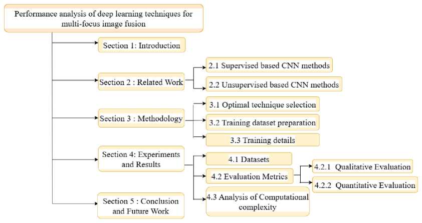
Fig.2. Organization of the paper

In this section, we delve into the realm of MFIF methods with a particular emphasis on exploring the advancements enabled by deep learning techniques. Establishing the basis for understanding the importance of deep learning in MFIF, the latest developments and trends have been discussed here.

Deep learning based MFIF methods are usually categorized into two types: supervised and unsupervised based CNN methods. Supervised techniques often need ground truth data for training, whereas unsupervised approaches do not require it. The two approaches have its own pros and cons persuading researchers to come up with new methods to handle issues of MFIF. These approaches frequently use deep learning models to improve fusion efficacy and produce better outcomes than conventional techniques.

Liu, Y. et al [10] introduced a pioneering approach using deep learning and CNNs for MFIF. CNN is trained to directly learn a mapping between source images and the focus maps. This addresses the issue of ALM and fusion rules which exists in traditional methods. It is a classification method where the input is given in the form of image patches, and it provides the result that whether the patch is focused or not. Nonetheless, eliminating a fully connected layer gave a negative impact on the performance. Additionally, the size of training patches causes inconsistencies along the boundary between clear and blurred areas.

Du, C. et al [20] has proposed image segmentation based MFIF approach named MSCNN to handle the issue of generating a decision map. To carry out image segmentation between clear and blurred region, the algorithm performs multi-scale analysis on every input image. But the max-pooling layer of CNN which is used for dimensionality reduction results in an information loss because of downsampling. This approach might be further developed to minimize information loss more effectively.

Tang, H. et al [8] introduces the use of deep CNNs for pixel-wise fusion (pCNN) of multi-focus images which identify clear and blur pixels in source images using information of adjacent pixels. It also builds an association between pixel wise and image-wise CNN demonstrating the possibility of transforming the pCNN to image-CNN for swift execution and it also minimizes the time complexity in MFIF.

Zhao, W. et al [21] proposed an end-to-end joint multi-level deeply supervised Convolutional neural network (MLCNN) in which both low-level and high-level features are integrated to extract distinct features from multi-focus images. This method shows great efficiency in handling input images characterized by unfocused regions, misregistration cases. Nevertheless, the method does exhibit a drawback when confronted with greatly mis-registered input images, leading to the introduction of certain artifacts.

Lai, R. et al [22] pr an end-to-end MFIF method named multi-scale visual attention deep convolutional neural network (MADCNN). The author designed two units- MFE unit and visual attention unit. Multi-scale feature extraction unit (MFE) is capable of gathering supplementary features from distinct spatial scales and merging them to effectively extract additional spatial information, consequently enhancing the precision of fusion. A visual attention unit aids the network in accurately identifying the concentrated region and choosing valuable features for the seamless integration of intricate details throughout the fusion procedure. In addition to this, the author suggests an artificial simulation method for generating multi-focus images; however, it may not entirely reflect the complexity and diversity of real-world multi focus scenarios.

Guo, X. et al [9] has developed a MFIF method based on fully convolutional network (FCN). It takes input as entire image where focus area is detected pixel by pixel, using trained FCN. The conditional random field (CRF) is employed to enhance focus region identification. However, the paper addresses that fusion quality can be enhanced by substituting Gaussian filter with deep neural network because they have powerful fitting capability to map between focus and defocus regions.

Amin-Naji, M. et al [18] has presented an ensemble learning method (ECNN) for MFIF to improve initial decision map and eradicate the demand for post-processing methods. Here three CNN models are trained on three different datasets (original, gradient in x and y direction) to develop primary decision map, giving rise to more accurate results than earlier approaches. The utilization of ensemble method has led to improved decision maps.

• Li, J. et al [17] has come up with a regression approach with pair learning named DRPL that transforms the complete image into binary mask using pixel-to-pixel regression, without any need of dividing it into patches. It addresses the challenge of predicting the degree of blur near focused and defocused boundary. It performs end-to-end training by generating the fused image directly from the predicted binary mask, thereby eliminating the need of post processing.

• 2.2.    Unsupervised based CNN Methods

Zhang, Y. et al [23] has presented a universal image fusion approach (IFCNN) designed as fully convolutional neural network which jointly optimizes all the parameters of model for the desired task, without any need for post processing. Here author make use of perceptual loss for the first time which helps improve the model to create additional texture aspect.

Xiao, Y. et al [24] developed degradation model based deep network (DMDN) that predicts the fully focused image from deteriorated images, rather than depending on focus map and post-processing approaches. Moreover, refraining from constructing intricate masks during training the network might have difficulty in properly handling complex defocus patterns or artifacts that may appear in real life scenarios. This constraint might influence network’s efficiency and capacity to generalize when confronted with a variety of potentially unanticipated defocused visual situations.

Mustafa, H. T. et al [25] designed a multi-level dense network (MLDNet) for MFIF where complex details from images are obtained by using dense connections. Firstly, at each level, local features are retrieved and fused, thereafter globally integrated to generate fused image which is then processed by reconstruction unit.

Xu, H. et al [26] has presented a MFIF method based on gradients and connected regions called GCF. Mask-net is designed to directly produces a binary mask, thereby overcoming the problem of vanishing gradient and eliminating the requirement for manually extracting the features or fusion rules. To achieve a more precise binary mask, the connected region numbers were employed as a constraint.

Xu, H. et al [27] come up with a unified architecture (U2Fusion) presented for various kinds of image fusion tasks, i.e multi-focus, multi-modal and multi-exposure image fusion, tackling the difficulties such as distinct solutions, storage, and computing constraints. Adaptive information preservation degree is used to extract features and retain information contained in the source images.

Jung, H. et al [28] proposed a deep image fusion network DIF-Net based on structure tensor representation. It basically demands the fused outcome to have the same contrast as input images having high dimensionality and no specific ground truth data is required. Fused images are produced through a single forward pass and loss function plays a major role here which makes the output similar to that of source images, by preserving the structural details.

Ma, B. et al [19] has presented an encoder-decoder architecture named SESF-Fuse to retrieve the actual input image. At the time of training, no fusion process is applied. At inference time, spatial frequency is used on the features extracted from encoder to determine their activity level. Specifically, this technique calculates gradient and use it to construct a decision map, as a result it is likely to recognize sharpest area having more gradient information, yet this technique is limited by its incapability to handle defocus spread effect. Moreover, there are inefficiencies in series fusion caused by decoder’s inability to reliably restore true pixel value leading to poor assessment of quality.

3.    Methodology 3.1.    Optimal Technique Selection

While there are numerous deep learning algorithms available for image fusion, the paucity of open source code for most of these algorithms is a major barrier to their acceptance and development of research in the area. Only few methods have their source code publicly available, due to which we are not able to compare sufficient number of approaches in this study.

So, we carefully selected three strategies ECNN [18], DRPL [17], SESF-Fuse [19] with easily available training source code for implementation and evaluation. Moreover, these techniques cover different learning paradigms like ECNN employs an ensemble of three CNNs to generate an initial decision map ensuring robustness in fusion, DRPL introduces a pair learning strategy to estimate binary maps corresponding to input images, thereby improving boundary consistency. In contrast to these two supervised methods, SESF-Fuse employs an unsupervised approach, utilizing an encoder-decoder architecture to learn fusion representations and extract deep features without the need for labeled data. The techniques having open source code promotes reproducibility and allows for an in-depth analysis of performance. This lays the framework for potential advances along with applications in MFIF with deep learning. An outline of above three techniques along with their link of source code is given in Table 1.

Table 1. Outline of techniques used in the study

Type Name of Technique Link of source code Supervised ECNN [18] DRPL [17] Unsupervised SESF-Fuse [19]

These techniques are described below.

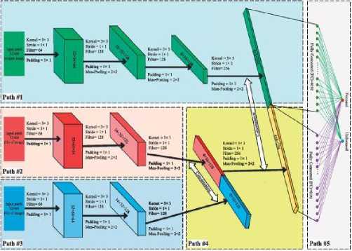
• •    ECNN [18] employs ensemble learning that is based on the utilization of three distinct CNN models, all of which have been trained on separate datasets. The aim of this approach is to attain an optimal initial segmented decision map. The architecture and the flowchart for ECNN are depicted in Fig.3a and Fig.3b respectively.

  

  (a). The network architecture of ECNN [18]

  Fig.3. ECNN architecture and its flowchart

  
  
  

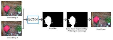
  (b). The flowchart of ECNN [18]

  
  

The functioning of the ECNN model involves the incorporation of both focused and defocused patches into the network which provides 0 or 1 labels corresponding to the focused and defocused regions, respectively. The architecture includes convolutional layers with a kernel of size 3 × 3, both stride and padding of size 1 × 1, ReLU activation along with max pooling of size 2 × 2. As shown in Fig.3a, the structure of ECNN consists of five paths: the first path takes the original dataset as input into the network, while Gx (gradient in horizontal direction) and Gy (gradient in vertical direction) datasets are passed through the second and third paths. The output of second and third paths is concatenated in the fourth path, which is then fused with the first path in the fifth one. In the end, a fully connected layer divides the output into two neurons for recognizing focused and defocused label [18]. After training, the fusion process in Fig.3b generates the score map by feeding overlapping patches of input images into the pre-trained network. Equation 1 outlines the fusion process for updating the score map, which evaluates each pixel multiple times. [18].

_ (M(i: i + b,j: j + b)+= -1   if label = 0

^(i,J) = ^{ M(i: i + b,j: j + b)+= 1   if label = 1

In the above equation, M(i,j) is the score map, where i is the row and j is the column of the source images. The dimensions of the extracted patches from the input images are indicated by the parameter b. The initial segmented decision map is obtained from M as given [18] below,

DM(i,j) = {1

if M^j) > 0 if else

where the decision map DM(i,j) is obtained through thresholding of M . The fused image is then generated using Equation 3 [18].

F(i,j) = DM(i,j)xA(i,j) + (1 — DM(i,jf)xB(i,j)

Here, F(i,j) is the final fused image, while A(i,j) and B(i,j) refers to the input multi-focus images [18].

In conclusion, the use of ensemble learning and simple structure of dataset improves the accuracy of decision map. The network design makes use of basic CNN models with small number of convolutional layers, with an emphasis on efficiency and simplicity in multi-focus image fusion tasks.

At first convolutional block, a large kernel of size 9 × 9 is used to increase the receptive field, then subsequently batch normalization layer, ReLU, and Swish activations as shown in Fig. 4a. The network then passes the input through two convolutional blocks with a kernel size of 3 × 3 prior sending it through 12 residual blocks to improve feature representation and reduce vanishing gradient problem. Following residual layers, the feature maps are passed through two successive convolutional layers and then final 3×3 convolution with Sigmoid is applied to ensure value of the output remains within [0,1]. Also, to preserve shallow features, skip connections are employed which improves performance. [17]. The fusion process of DRPL as shown in Fig.4b, commences by inputting a pair of complementary input images into a fully convolutional network, to determine their associated weighted maps. These maps are then combined using dot product and weighted summation method to generate the fused image as shown in Equation 4 [17].

I_f = I_a О f(I_a)+ I_b О f(I_b) (4)

where I_a and I_b are the input images, f(I a ) = f-f i l+l—lflJ i l and f(I_b) = 1 — f(I_a) and О denotes the dot product, The purpose of this procedure is to guarantee that the weighted binary maps are complementary to each other i.e. the focused part in one image is defocused in another image and vice-versa [17].

In summary, this method is based on pair learning approach that estimates binary masks from complementary source images which leads to improved quality of fused image, eliminating the need of dividing the source images into patches, demonstrating the practicality and superiority of the approach [17].

SESF-Fuse [19] is an unsupervised technique where a network consisting of an encoder and decoder is trained to get deep level features from input images [19]. The SESF architecture can be seen in Fig.5. The encoder incorporates five successive convolutional layers, where the output of each layer is connected to the other layers. It improves the feature transmission and reduces the number of parameters. To ensure image reconstructs accurately, no pooling layers are used.

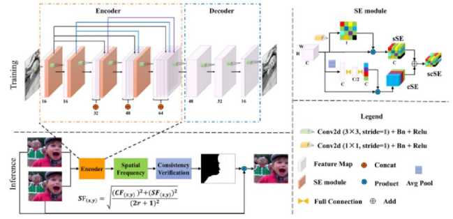
Fig.5. The framework of SESF [19]

Further, the robustness and accuracy of deep features is enhanced using three forms of SE (Squeeze and Excitation) module - sS E1, cS E2, scS E3. sSE refine features based on spatial information using 1 × 1 convolution and cSE captures global spatial information using average pooling and two fully connected layers to improve channel-wise dependencies. scSE combines both of them element-wise to refine feature learning in both channel and spatial direction. Finally, the decoder reconstructs the input image using four convolutional layers. In the inference phase, spatial frequency (SF) is applied to the deep features extracted from encoder to compute an initial decision map, which reflect the activity levels. The initial decision map D^ j) , is obtained as shown below [19]:

_D- f ¹     V ^SF1(i,i) > ^SF2(i,i)

1,1     (.0                other-wise where (i,j) are the coordinates of the feature vector in deep features. Subsequently, to obtain final decision map, a guided filter is utilized as a means of consistency verification to mitigate any undesired artifacts around the boundary between the clear and blurred areas. The fused image is then produced using a pixel-wise weighted fusion rule as

^F(i,i) = ^D(i,i)^lm 3 ^A(i,i) ^{+ (1- D}(i,i) ) ^lm B ^B(i,i)

where lmgA and lmgB are source images, D ( _l i) is the decision map based on spatial frequency of both source images [19].

To sum up, this method assesses sharp instances in deep features of input images using SE module and then apply SF to determine the activity level using those deep features to generate a decision map. As a result, it is more likely to identify clarity regions that seem crisp and include more gradient information.

To ensure that the existing fusion models are resilient and generalizable, we trained them on three different datasets. The strategy for preparing the dataset is discussed in next subsection.

• 3.2.    Training Dataset Preparation

In the domain of MFIF, a significant obstacle is the lack of adequate datasets and its ground truth labels which leads to the challenge of generating extensive datasets. Although many datasets are available in literature such as RealMFF [1], Lytro dataset [29], MFFW dataset [30], MFI-WHU dataset [31] and many more, but still they lack the availability of sufficient image pairs required for accurate training and assessment. Even some of them are not publicly available. To deal with this inadequacy, the researchers often generate synthetic datasets by intentionally applying Gaussian blur to make the ultimate images seems like natural ones. Though this strategy is not desirable, it assists to eliminate the dataset bottleneck and allows for training of fusion algorithms on a wider variety of image variations.

Following that, synthetic dataset using gaussian blur is generated using the strategy given by the respective authors of selected three MFIF techniques. The synthetic data generation method was adjusted to each respective technique, to make sure the training process met the unique needs thereby enhancing their ability to learn distinct characteristics and capture the intricacies of MFIF methods. For training of multi-focus images, we utilized the most widely used datasets in computer vision namely, ILSVRC2012 [32], COCO2017 [33], and DIV2K dataset [34].

Since these datasets do not contain multi-focus images naturally and as we need high quality focused images to generate multi-focus images, we utilize the dataset generation method specified in the respective techniques. Each dataset offers distinct properties that help in the development of learning robust focus-related characteristics.

ILSVRC2012 dataset consists of 1.2 million high-quality focused images across 1000 categories for image classification and object recognition [32]. COCO2017 is also an extensive dataset for object detection and segmentation task consisting 330K images over 80 object categories [33]. The DIV2K dataset also captures high-quality focused images with complex details, rich textures, and varied lighting scenarios created for a super-resolution task involving 1000 RGB images. These images are 2K resolution, meaning they have 2K pixels on atleast one of the axes either horizontal or vertical [34].

These datasets were selected only for their fully focused images, which we use to generate synthetic multi-focus image pairs using Gaussian blur. Since ILSVRC2012 and COCO2017 had large number of images, DIV2K did not possess sufficient images. To solve this issue, data augmentation has been applied to DIV2K dataset to generate requisite number of images to generate enough number of pairs. Data augmentation such as flipping the images horizontally and vertically, rotating at 20°, 40°, 90°, 120°, 200°, 270°, 330°, 360° are applied to increase the no. of images required for training.

The methodology to make the dataset for each technique is discussed below.

• •    For ECNN, the training dataset is constructed using 1040 images of high-quality from the respective dataset. These images are converted to grayscale and undergo Gaussian filtering with a standard deviation of 9 to simulate four levels of blur. These four levels are 9 × 9, 11 × 11, 13 × 13 and 15 × 15. Consequently, five types of images are obtained: the original image and four versions of blurred images. The gradient is then applied in the horizontal and vertical directions to generate three groups of images: original images, Gx (gradient in horizontal direction), and Gy (gradient in vertical direction) datasets. Each image is divided into 32 × 32 patches, where each patch represents either a clear (non-blurred) image or one of the four blurred types. These patches are vertically concatenated to form 64 × 32 macro-patches. If the upper half of a macropatch is from the clear version and the lower half is from one of the four blurred versions, it is labeled as upper focused data (0). Similarly, if the upper half is from the blurred version and the lower half is from the clear version, it is labeled as lower focused data (1). This process generates 1,02,400 macro-patches for training and 30,720 patches for validation per dataset [18].

• •    For DRPL technique, a total of 1040 focused images from the respective dataset were utilized to construct the training dataset. These images underwent cropping to obtain sub-images with dimensions of 256 × 256 from their central regions. From each sub-image, 9 sub-patches of size 128 × 128 were cropped with a fixed stride of 64, resulting in a total of 9360 images. To generate blurred images with varying levels of blur, Gaussian filtering was applied with a standard deviation of 1.5 and a cutoff of 7x7. Consequently, for each sample, there was one focused image and three blurred images. The initial blurred image was generated by applying a Gaussian filter to the original clear image. Subsequently, the second blurred image was generated from the first blurred image using the same filter, followed by the creation of the third blurred image. These original and blurred images were then combined to create more challenging training images. To achieve this, 213 pairs of binary masks, as provided in the paper by the author of this technique, were used [17]. Given a pair of focused and defocused images, a multi-focus image pair was generated using a following equation [17].

la~ I dear ^О M a + ¹ blur ^{О M} b ! b ~! clear О ^M b + ^ blur ^ ^M a

where I_clear and 1_Ыиг represent the clear and blurred images. M_a and M_b denote the complementary masks, which are randomly selected to form pairs. In this manner, a total of 28,080 pairs were generated, out of which 20,000 pairs were utilized for training and the rest of the pairs for validation [17].

• •    For SESF-Fuse, being an unsupervised approach, no ground truth is used. The author employs all-clear focused images to train encoder-decoder architecture. Specifically, 20,000 images are arbitrarily selected from the respective dataset for training, while another 8080 images are used for validation purposes [19].

• 3.3.    Training Details

  In this work, the idea of transfer learning is used to train three techniques across three different datasets. Transfer learning involves fine-tuning weights from previously learned model on a huge dataset for a particular task, like in our case it is MFIF. We used this concept for all the three approaches exploiting the weights provided by the developers to train and fine-tune the image fusion algorithms on ILSVRC, COCO and DIV2K dataset. This approach allowed us to delve into the information and interpretations obtained from the larger dataset, thereby enhancing the capability of fusion models to identify key patterns and characteristics for MFIF. While default parameters reported by the authors were utilized, adjustments were made to the number of epochs and batch size according to the available RAM and GPU capacity. However, a thorough evaluation of hyper-parameter influence is not done as focus was to ensure fair comparison among techniques using the default settings provided in the paper. All the experiments were performed on NVIDIA RTX4000 with 32GB RAM. Table 3 shows the training details for each of the three techniques.

4.    Experiments and Results 4.1.    Datasets

By following the dataset generation process, we ensured that it meets the specific needs of each method. These personalized approaches enabled us to efficiently train and evaluate existing image fusion techniques hence improving the reliability and efficacy of our research outcomes. The number of training and validation images used for every technique along with input image resolution is shown in Table 2.

Table 2. Description of number of images/patches and input resolution used for training

Name	No. of training images/ patches	No. of validation images/ patches	Input resolution of images/ patches
ECNN [18]	1,02,400 patches	30,720 patches	32 × 64
DRPL [17]	20,000 pairs	8080 pairs	128 × 128
SESF-Fuse [19]	20,000 images	8080 images	256 × 256

Table 3. Training details for each technique

Hyperparameter	Technique
	ECNN [18]	DRPL [17]	SESF-Fuse [19]
Optimizer	Stochastic Gradient Descent	Adam	Adam
Learning rate	0.0002	0.001	0.0001
Weight decay	0.0005	0.5	0.8
Scheduler	StepLR	StepLR	-
Gamma	0.9	0.5	-
Batch-size	8	16	12
No. of Epochs	50	50	30
Loss	Cross Entropy Loss	L1 loss	SSIM and Pixel loss

To compare performance comprehensively, two widely used MFIF datasets were employed, namely Lytro dataset [29] and RealMFF dataset [1]. Both datasets are captured with light-field camera containing diverse multi-focus scenes at different focus depths. Lytro dataset [29] consists of 20 pairs of color multi-focus images while RealMFF [1] comprises 710 pairs with ground truth images. In this study, all the 20 pairs from Lytro dataset were utilized and 10 pairs were randomly selected from RealMFF dataset for evaluation. A brief description about these datasets is given in the Table 4. All the image pairs are pre-registered.

Table 4. Description of datasets used for evaluation

Name No. of pairs Resolution Ground truth Source link Lytro [29] 20 520 × 520 No RealMFF [1] 710 625 × 433 Yes

• 4.2.    Evaluation Metrics

Evaluation metrics are critical in determining the effectiveness of MFIF. But, as there is no ground truth available in MFIF datasets, so assessing the quality of these algorithms is difficult. The analysis of fused images normally takes two forms: qualitative evaluation and quantitative evaluation. These are explained as below.

• A . Qualitative Evaluation

Qualitative evaluation commonly referred to as subjective evaluation, depends on human observation to measure visual performance of fused images, yielding meaningful perspective in MFIF domain. Despite that, it has some drawbacks such as, it is laborious and susceptible to prejudiced judgment because of varying observer criteria, determining visual information with bare eyes is hard, and so individuals must have appropriate professional experience.

Furthermore, external factors such as illumination and brightness also impact observer’s decisions. Several evaluation sessions need to be conducted to bring accuracy. As a result, subjective evaluation is supplemented with objective evaluation measures [35, 36].

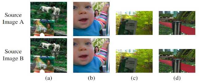
Fig.6. Source image pairs employed to visually illustrate the results

• a.    Discussion on Results when Trained on ILSVRC2012 and Tested on Lytro Dataset

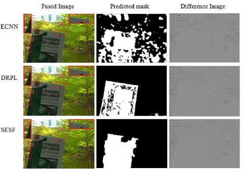
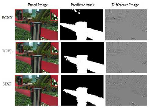
In Fig.7a, the results of Fig.6(a) are visually depicted. By examining, it can be observed that the fused image generated by the ECNN method displays certain imperfections along the edges of the boundary region. The edges and corners lack precise definition and appear more rounded, as supported by the mask and difference image. Conversely, the DRPL and SESF methods exhibit superior performance when compared to the ECNN method. However, it is noteworthy that SESF results in a loss of detail around the left bottom corner. These observations are further substantiated by the areas in the mask and difference images corresponding to highlighted area in fused image.

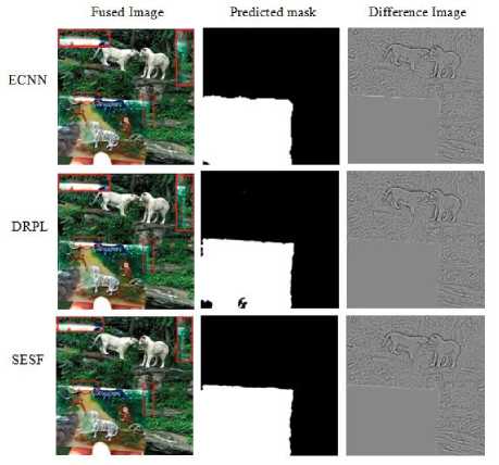
(a) Results on Source Image A and B on Fig. 6(a)

Fig.7. Results on Lytro dataset when trained on ILSVRC2012

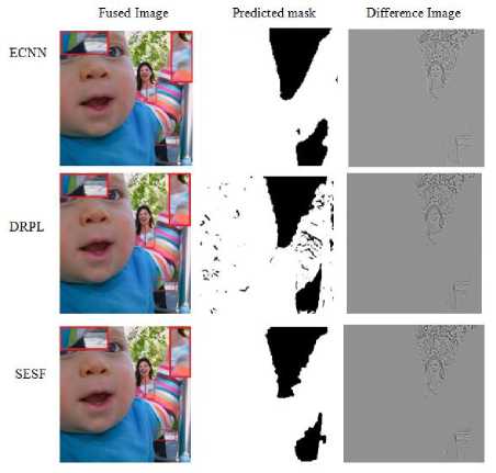
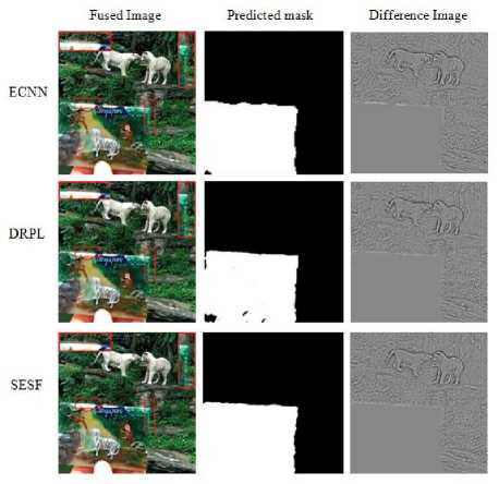
(b) Results on Source Image A and B on Fig. 6(b)

Fig.7b shows the findings for the pair represented in Fig.6(b). It is worth noting that the ECNN method demonstrates a limitation in its ability to accurately detect corners, as evidenced by the rounded shape observed in both its fused image and mask. Also, there is loss of information at the edge of infant’s face. The DRPL approach produces residuals in the focal region. While the SESF approach produces a visually appealing appearance, it loses clarity around the infant’s arm due to some misclassified pixels and injection of noise at the margins.

• b.    Discussion on Results when Trained on ILSVRC2012 and Tested on RealMFF Dataset

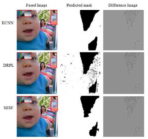
In Fig.8a, the outcomes of the RealMFF pair depicted in Fig.6(c) are exhibited. Here, DRPL surpasses both ECNN and SESF in visual performance. It effectively produces clearest edge details. However some blurred areas are present in the focused region. SESF also excels in information preservation, but edges are not well defined. It introduces some artifacts around the edges of book as can be seen from difference image and zoomed part also. The selected region shows that there is blurriness around the top edge of the book. For ECNN, some regions from both source images did not merge well in fused image, blur artifacts are visible in the fused image as well as difference image.

In Fig.8b, the outcomes of Fig.6(d) are illustrated. ECNN operates effectively but some residuals can be seen in the background. Furthermore, the contour details are unsatisfactory. Fused image of both DRPL and SESF fails to capture focus details at the left of the carpet as seen from the mask also. SESF betrays blur artifacts on boundary region on the right of lamp.

(a) Results on Source Image A and B on Fig. 6(c)

Fig.8. Results on RealMFF dataset when trained on ILSVRC2012

(b) Results on Source Image A and B on Fig. 6(d)

• c.    Discussion on Results when Trained on COCO2017 and Tested on Lytro Dataset

  

  (a) Results on Source Image A and B on Fig. 6(a)

  
  

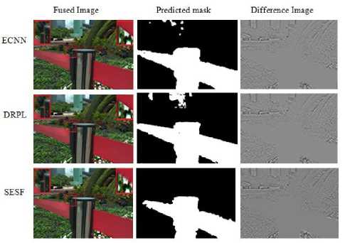
  Fig.9a illustrates the results of Fig.6(a) pair. Here all three techniques exhibit noticeable artifacts in the boundary region. ECNN has some contrast at focused and defocused boundary. DRPL and SESF preserve details of focused region however there are slight artifacts at the boundary which can be clearly seen from their corresponding difference image.

  

  (b) Results on Source Image A and B on Fig. 6(b)

  
  

  Fig.9. Results on Lytro dataset when trained on COCO2017

• d.    Discussion on Results when Trained on COCO2017 and Tested on RealMFF Dataset

  Fig.10a, the results of 6(c) are represented. DRPL performs well at the boundary, although minor artifacts can be seen at the left edge of the book. ECNN lacks boundary details around the book. SESF encounters difficulty in detecting the boundary at the top, leading to blurriness in that region. Furthermore, a contrast is also observed in the highlighted area on the left edge of the book.

  The results of Fig.6(d) are visualized in Fig.10b. ECNN preserved detailed information, but artifacts are present, around the boundary regions. There is also a slight increase in the contrast. In both DRPL and SESF, fused information from both source images do not merge well. SESF produces artifacts on the FDB on the right side of lamp highlighted red box. It can be clearly seen from difference image as well.

  

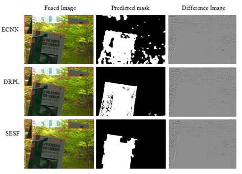
  (a) Results on Source Image A and B on Fig. 6(c)

  
  
  

  (b) Results on Source Image A and B on Fig. 6(d)

  
  

  Fig.10. Results on RealMFF dataset when trained on COCO2017

• e.    Discussion on Results when Trained on DIV2K and Tested on Lytro Dataset

In Fig.11a, the results of Fig.6(a) are given. ECNN produces undesirable artifacts at the boundary region. In SESF, rippling artifacts appeared at the vertical edge of the picture. DRPL loses some details around boundary region.

Moving on to Fig.11b, the results of Fig.6(b) are visualized. In ECNN, blur artifacts can be easily seen in the region below the infant’s arm (see the difference image and the area highlighted by the red rectangle.) DRPL shows significantly fewer residuals in the focused part compared to Fig. 7b and 8b. However, noise is introduced at the edge of the infant’s arm and face. The highlighted area in the fused image exhibits distortion and blurriness. Although SESF achieves better results in terms of information retention, as can be observed from the fused image, it still produces noise around the infant’s arm.

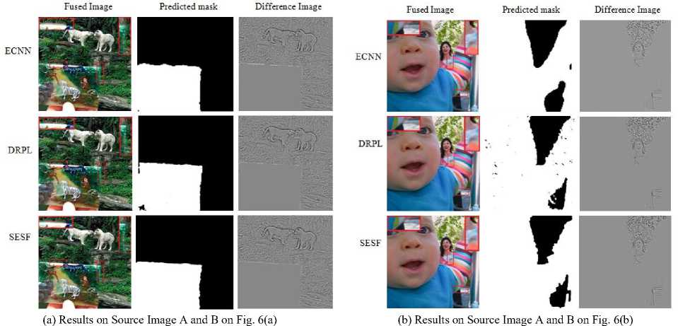
Fig.11. Results on Lytro dataset when trained on DIV2K

• f.    Discussion on Results when Trained on DIV2K and Tested on RealMFF Dataset

Fig.12b shows the results of Fig. 6(d) all techniques perform satisfactorily. In ECNN, fusion does not happen properly around the boundary region. Edges are not precise and moreover they appear rounded at the corners. SESF does not differentiate between clear and blur at left corner of carpet, boundary regions depict loss of information. DRPL performs well, have precise boundary edges, however slight residuals are present around the lamp.

(a) Results on Source Image A and B on Fig. 6(c)

Fig.12. Results on RealMFF dataset when trained on DIV2K

(b) Results on Source Image A and B on Fig. 6(d)

• B . Quantitative Evaluation

Objective evaluation comes into practice where evaluation of fused image does not require ground truth. Here the quality of image is assessed based on contrast, brightness and information retention. Both subjective and objective evaluations help to provide complete knowledge of MFIF techniques. Liu et al. [37] classified twelve prominent image fusion metrics into four groups: information theory-based, image feature based, image structural similarity based, and the human perception inspired metrics. In our experiments, one metric that is broadly used in MFIF is employed for evaluation from each group. These metrics are Mutual information [38], Gradient based metric [39], Piella metric [40], Chen-Varshney metric [41] respectively.

• •    Mutual Information (Q MI ): It estimates the quantity of information transmitted to the fused image from the input images [38]. It is obtained using the formula shown below:

  Г ^MI(AF

  ^^MI   2 ^[ H(A) + H(F)

  
  

  MI(B,F) H(B)+H(F)

  
  

  _:]

  
  
  
  

where A, В are two source images, В is the fused image, MI(A, F) is the mutual information between two images A and F . H(A), Н(В) and H(F) are the entropies of image A, В and F. Higher the MI value, greater the quality of image fusion, ensuring better information transfer. The same explanation applies for MI(B, F) [38].

• •    Gradient based metric (Q^AB/F): This is an edge based similarity measurement metric given by [39] which describes the quantity of edge information aired from source images to the fused image. It is calculated as:

X n=₁ T m=₁ Q^AF( ⁿ ,m)w^A(n,m) + Q^BF (n,m)w^B(n,m) T ^l j ^F^^^

where N x M is the image size, Q^AF(n, m) is the edge information preservation value and it is defined by the product of two factors: Q g ^F(n,m). Q^AF(n,m). These variables indicate the edge strength and orientation information value preserved at position (n,m). The value of Q^AF(n,m) ranges from 0 to 1, with 0 indicating that no edge information is transferred from source image A to F at given location (n, m) whereas value of 1 indicates considerable fusion from A to F with no loss of information. The same applies for Q^BF(n,m) as well. The weighting factors w^A(n,m) and w^B(n,m) represents the importance of Q^AF(n,m) and Q^BF(n,m) respectively [39].

• •    Piella metric (Q E ): Piella and Heijmans [40] presented three fusion quality indicators using Wang’s UIQI (universal image quality index) approach. This metric shows how much structural information has been transferred from input images to the fused image.

The fusion quality index is defined as

Q s = ^Z_W ew [A(w)Q ₀ (A,F|w) + (1-A(w))Q₀(B,Flw)]                    (10)

The weighted fusion quality index is calculated as

^Qw Е шеЖ c(w)\A(w)Q₀(A,Flw) + (1-A(w))Q ₀ (B,F|w)]

Now, let A' , B' and F' are the edge images of A , В and F . Then the edge-dependent fusion quality index is calculated as

Q e = Q w (A,B,F^.Q w (A',B',FT

where Q(A,B|w) is a local quality index, calculated in a sliding window w. A(w) is the saliency weight derived using the variances of input images. c(w) is the normalized saliency of window across all the local windows. a is a manually adjustable parameter that quantifies the contribution of edge images in comparison to original images. [2, 40].

• •    Chen-Varshney metric (Q CV ): The method Q CV [41] analyzes the visual contrast between the input images and the fused image, without the need of ground truth. It is broken down into 5 stages: retrieving edge details, dividing image into local areas, determining saliency of local region, assessing local similarity and evaluating global quality. The global quality index is then determined as the weighted sum of all the local windows as

i !.₁ (ow)’‘(-M'';¹)) й ., (< ‘ )+<■))

where D (I™¹ . I^w ) and D (I™¹ . I™¹} is the similarity measure between the source and the fused image computed as mean squared value using contrast sensitive filtered images. A(l^W ‘ ) and A(l^W ‘ ) are the local saliency of source images. The value of Q_cv lies in the range of 0 to ». Lower the value, better the quality of fused image [41].

Table 5. Average values of all three MFIF methods on Lytro dataset (20 pairs) and Real-MFF dataset (10 pairs)

Method	Trained on Dataset	Lytro Dataset				RealMFF Dataset
		Q MI	Q AB/F	Q E	Q CV	Q MI	Q AB/F	Q E	Q CV
ECNN	ILSVRC2012	1.0840	0.7024	0.9379	16.5410	1.1617	0.6635	0.9248	50.4489
	COCO2017	1.0853	0.7030	0.9381	16.4962	1.1706	0.6835	0.9355	46.4642
	DIV2K	1.0857	0.7032	0.9381	16.7295	1.1760	0.6976	0.9426	44.4507
DRPL	ILSVRC2012	1.0084	0.7133	0.9447	16.0041	1.1895	0.7437	0.9645	41.0871
	COCO2017	1.0051	0.7120	0.9447	16.3126	1.1851	0.7446	0.9648	42.9568
	DIV2K	1.0043	0.7104	0.9444	16.0572	1.1725	0.7161	0.9547	44.2858
SESF-Fuse	ILSVRC2012	1.0391	0.7228	0.9452	16.0282	1.1674	0.7407	0.9639	39.5738
	COCO2017	1.0390	0.7227	0.9452	16.0381	1.1676	0.7408	0.9639	39.9467
	DIV2K	1.0389	0.7226	0.9452	16.0138	1.1677	0.7409	0.9640	40.1912

In this work, we use the toolki t4 designed by the initial author of [37] for objective assessment and all the default values were used as stated in the relevant articles. Table 5 compares the objective performance of three fusion methods using four metrics on Lytro and RealMFF dataset. The average scores on 20 pairs from Lytro dataset and 10 pairs from RealMFF dataset for each approach are given. The best three values on each metric are shown in bold for both datasets.

ECNN shows moderate performance across all metrics and training datasets. ECNNs higher Q CV values imply that it did not perform well in content visualization compared to other approaches. Also, it exhibits lower Q^AB/F and Q E values, showing a lack of edge information as well as structural similarity transferred to the fused image which are crucial for high-quality image fusion.

DRPL performs consistently across datasets. For RealMFF dataset, DRPL achieves high Q MI , Q AB/F and Q E scores, indicating higher fusion quality for information transfer, image feature preservation, and structural similarity. It also exhibits lower Q CV values when trained on ILSVRC2012, resulting in improved content visualization quality.

SESF performs consistently and competitively across several datasets. It shows good performance on Lytro dataset in terms of Q AB/F and Q E scores, showing efficient gradient information transmission and picture quality retention. In addition to this, it also produces lower Q CV values than other approaches on both lytro and RealMFF dataset. This demonstrates that SESF performs considerably better in terms of content visualization quality.

The findings highlight the need of using different assessment measures to properly analyze fusion quality. As can be observed, every algorithm performs differently on various metrics, demonstrating that these algorithms are capable of dealing with diverse types of information. Although ECNN do not excel in every parameter, but overall, it performs well across all the four metrics.

• 4.3.    Analysis of Computational Complexity of MFIF Techniques

5.    Conclusions and Future Scope

The computational complexity of three techniques as shown in Table 6 is compared with four different aspects: (i) average running time (in sec) to generate a fused image on both Lytro and RealMFF dataset, (ii) FLOPs (in GB) denotes the floating point operations, (iii) parameter size (in MB) and (iv) total parameters (in millions).

Table 6. Average values of all three MFIF methods on Lytro dataset (20 pairs) and Real-MFF dataset (10 pairs)

Technique	Average running time (sec)		Training cost
	Lytro Dataset	RealMFF Dataset	FLOPs (G)	Parameter size (MB)	Parameters (M)
ECNN [18]	0.1927	0.1874	0.799	6.05	1.58
DRPL [17]	0.2235	0.2636	288.57	4.28	1.07
SESF-Fuse [19]	0.3366	0.4148	20.06	0.30	0.07

Among the three methods, ECNN is the most computationally efficient since it produces the fastest inference with least FLOPs. In spite of DRPL’s greater parameter efficiency, it shows noticeably larger FLOPs, suggesting a trade-off between computational demand and model’s complexity. On the other hand, SESF-Fuse has the longest inference time despite having fewest parameters.

So, every method has shown some strengths and limitations. ECNN on one hand uses ensemble model which shows great results in producing accurate initial decision map and hence the fused image, but on the other hand, it follows a patch based strategy where diving an image into patches leads to inconsistencies around the boundary region. However, integrating mechanisms like global contextual awareness and boundary handling mechanisms can contribute to achieve better fusion quality. While DRPL has ability to fuse complementary multi-focus images, some misclassified areas impact the quality of fusion. So, it may face challenge in retaining accurate information from source images for which some attention mechanisms are required to enhance performance. SESF-Fuse, on the other hand, cannot handle defocus spread effect which leads to information loss at the boundary area. Although it maintain clarity in the fused image, yet its performance could be further improved by adopting advanced gradient computation methods to replace traditional spatial frequency approaches, potentially leading to better edge preservation and overall fusion quality.

This study analyzes the performance evaluation of three deep learning based MFIF techniques. Both qualitative and quantitative experiments were performed to determine the effectiveness of these MFIF techniques on Lytro and RealMFF datasets using four objective assessment measures, offering in-depth analysis of their fusion abilities. Our thorough research and experiments aim to provide valuable insights into the strengths and limitations of current deep learning based MFIF techniques, ultimately advancing the field.

The utilization of transfer learning expedited the convergence, boosted overall performance, and facilitated the adaptation of fusion models to the distinct features found in the ILSVRC, COCO, and DIV2K datasets. The applications of MFIF techniques have immense potential in various domains including surveillance, robotics, remote sensing and medical imaging. By effectively integrating information derived from images taken at various focal planes, MFIF enhances the clarity and detail of the image, thus facilitating better decision-making and analysis in these areas.

In future, research in the field of MFIF could explore the incorporation of innovative network architectures specifically tailored for this task, further enhancing fusion quality and preserving intricate image details. Efforts to enhance the computational efficiency of MFIF techniques for real-time implementation offer promising future prospects. Moreover, a possible research area of this study can be to analyze the impact of hyper-parameter modifications like batch size, learning rate, etc. which would enable these techniques to be further optimized for various applications and datasets.

By leveraging these opportunities, we can lay the groundwork for the advancement of more intricate and adaptable fusion methodologies that more effectively address the requirements of practical applications.

Acknowledgements

This research is supported by University Grants Commission (UGC), New Delhi (India).