Performance Analysis of Resampling Techniques on Class Imbalance Issue in Software Defect Prediction

Автор: Ahmed Iqbal, Shabib Aftab, Faseeha Matloob

Журнал: International Journal of Information Technology and Computer Science @ijitcs

Статья в выпуске: 11 Vol. 11, 2019 года.

Бесплатный доступ

Predicting the defects at early stage of software development life cycle can improve the quality of end product at lower cost. Machine learning techniques have been proved to be an effective way for software defect prediction however an imbalance dataset of software defects is the main issue of lower and biased performance of classifiers. This issue can be resolved by applying the re-sampling methods on software defect dataset before the classification process. This research analyzes the performance of three widely used resampling techniques on class imbalance issue for software defect prediction. The resampling techniques include: “Random Under Sampling”, “Random Over Sampling” and “Synthetic Minority Oversampling Technique (SMOTE)”. For experiments, 12 publically available cleaned NASA MDP datasets are used with 10 widely used supervised machine learning classifiers. The performance is evaluated through various measures including: F-measure, Accuracy, MCC and ROC. According to results, most of the classifiers performed better with “Random Over Sampling” technique in many datasets.

Еще

Software Defect predication, Imbalanced Dataset, Resampling Methods, Random Under Sampling, Random Oversampling, Synthetic Minority Oversampling Technique

Короткий адрес: https://sciup.org/15017086

IDR: 15017086 | DOI: 10.5815/ijitcs.2019.11.05

Текст научной статьи Performance Analysis of Resampling Techniques on Class Imbalance Issue in Software Defect Prediction

Published Online November 2019 in MECS DOI: 10.5815/ijitcs.2019.11.05

Developers and researchers have always been concerned to develop high quality softwares at lower cost [7, 8, 9]. Predicting the defects at early stage of development life cycle can achieve this goal as the cost of fixing the defects increases exponently at later stages [8], [20, 21]. Software defect prediction is the problem of binary classification in which we have to classify the particular module as defective or non-defective [7, 8, 9]. Supervised machine learning techniques have been widely used to solve the binary classification problems such as Sentiment Analysis [12, 13, 14, 15], Rainfall Prediction [16, 17], and DoS attack detection [18, 19]. The supervised machine learning techniques uses preclassified data (training data) in order to train the classifier. During the training process, classification rules are developed which are used to classify the unseen data (test data) [10, 11]. The datasets of software defects are usually skewed in which too many instances are related to one class and very less instances belong to second class. For instance, normally less records are related to defective class and too much records are related to nondefective class. The class with less instances is known as minority class and the class with the too many instances is known as the majority class. The imbalance between these two classes is reflected by “Imbalance ratio”, which is the ratio of the number of instances in majority class to that of a minority class. [1]. In software defect datasets, the instances related to non-defective class are usually high with respect to defective instances as shown in this table 1. Therefore the particular classifiers trained on such imbalanced datasets may produce the bias result and may classify the minority instance as majority instance. To resolve this issue, many techniques are available. This paper uses three well known resampling techniques to handle the class imbalance issue for software defect prediction. The resampling techniques include: Random Under Sampling (ROS), Random Over Sampling (RUS) and Synthetic Minority Oversampling Technique (SMOTE). Twelve (12) publically available cleaned NASA MDP datasets are used for experiments along with 10 widely used supervised machine learning classifiers including: “Naïve Bayes (NB), Multi-Layer Perceptron (MLP). Radial Basis Function (RBF), Support Vector Machine (SVM), K Nearest Neighbor (KNN), kStar (K*), One Rule (OneR), PART, Decision Tree (DT), and Random Forest (RF)”. Performance evaluation is performed by using: “F-measure, Accuracy, MCC and ROC”. The results reflects that ROS performed better in almost all the datasets.

The rest of the paper is organized as follows: Section 2 discusses the related work done on Class Imbalance issue. Section 3 elaborates the materials and methods which are used in this research. Section 4 reflects the results of experiments. Section 5 finally concludes this research.

II. Related Work

Many researchers have worked to resolve the class imbalance issue since the last decade. Some of the related studies are discussed here. In [1], the authors proposed SOS-BUS which is a hybrid resampling technique. This approach integrated a well- known oversampling technique SMOTE with the newly developed Under Sampling Technique. The proposed approach focusses on the necessary data of majority class and avoid the removal stage from random under-sampling. The results reflected that the proposed technique performed better in Area under ROC Curve (AUC). In [2], the researchers discussed class imbalance learning methods and elaborated that how these methods can be used for effective software defect prediction. They investigated various class imbalance learning methods such as resampling techniques, threshold moving techniques, and ensemble algorithms. AdaBoost.NC reflected high performance in Balance, G-mean, and Area Under the Curve (AUC). Moreover an improvement in AdaBoost.NC has also been proposed in which parameter adjustment is performed automatically during the training process. The proposed version proved to be more effective and efficient. Researchers in [3] discussed two resampling techniques which are the extensions of SMOTE and RUS. They have studied and discussed an ensemble learning method AdaBoost.R2 to resolve the data imbalance issue for software defect prediction. The researchers discussed that the extensions of SMOTE and RUS, SmoteND and RusND are the effective techniques to resolve the imbalance issue in software defect datasets. Experiments on 6 datasets with two performance measures have showed the effectives of these techniques. Moreover in order to improve the performance of these techniques, AdaBoost.R2 algorithm is integrated and made these techniques as SmoteNDBoost and RusNDBoost. Experiments reflected that the hybrid approach outperformed the individual techniques including SmoteND, RusND and AdaBoost.R2). Researchers in [4] analyzed the performance of SMOTE on the issue of class imbalance on software defect prediction. They have analyzed that at which extent the SMOTE technique can improve the classification of defective software modules. The researchers reflected that after applying the SMOTE technique the dataset became more balanced and more accurate results were noted on four benchmark datasets. In [5], the researchers have proposed a software defect prediction system named “Weighted Least Squares Twin Support Vector Machine” (WLSTSVM). The proposed system works by assigning the higher misclassification cost to the instances related to defective class and lower cost to the instances related to non-defective class. Experiments were performed by using 8 software defect datasets which showed that the proposed system performed better in non-parametric Wilcoxon signed rank test. Researchers in [6] used three re sampling techniques on credit card dataset in order to overcome the class imbalance issue. The techniques include: Random Under Sampling, Random Over Sampling and Synthetic Minority Oversampling Technique. The performance was evaluated by using Sensitivity, Specificity, Accuracy, Precision, Area Under Curve (AUC) and Error Rate. The results reflected that the resampled datasets brought better performance. Researchers in [7] analyzed the performance of various widely used supervised classifiers on software defect prediction. For experiments, 12 publically available NASA datasets were used. The classification techniques included: “Naïve Bayes (NB), Multi-Layer Perceptron

(MLP). Radial Basis Function (RBF), Support Vector Machine (SVM), K Nearest Neighbor (KNN), kStar (K*), One Rule (OneR), PART, Decision Tree (DT), and Random Forest (RF)”. The performance is evaluated by using Precision, Recall, F-Measure, Accuracy, MCC, and ROC Area. The researchers have observed that that neither the Accuracy and nor the ROC can be used as an effective performance measure as both of these did not react on class imbalance issue. However, Precision, Recall, F-Measure and MCC reacted to class imbalance problem in the results.

III. Materials and Methods

This research aims to analyze the performance of three well known resampling techniques on class imbalance issue for software defect prediction. For this purpose a comparison framework (Fig. 1) is used in which performance of each re-sampling technique is analyzed with various well known classifiers. The framework consists of four stages: 1) Dataset selection, 2) Resampling, 3) Classification, and 4) reflection and analysis of Results. First stage deals with the selection of datasets in which 12 cleaned NASA MDP datasets are used for experiments including: “CM1, JM1, KC1, KC3, MC1, MC2, MW1, PC1, PC2, PC3, PC4 and PC5 (Table I)”. Each of the used dataset represents a particular NASA’s software system. The datasets include various quality metrics in the form of attributes along with known output class. The output class is also called the target class which is predicted on behalf of other attributes. The attribute which holds the target/output class is known as dependent attribute and other attributes are known as independent attributes as those are used to predict the dependent attribute.

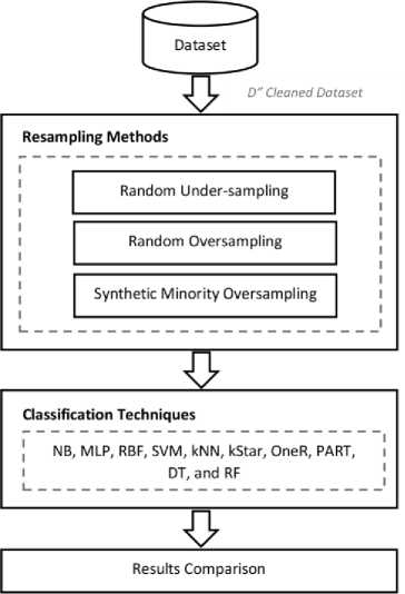
Fig.1. Comparison Framework

Table 1. Cleaned NASA Software Datasets [22], [23]

Dataset	Attributes	Modules	Defective	NonDefective
CM1	38	327	42	285
JM1	22	7,720	1,612	6,108
KC1	22	1,162	294	868
KC3	40	194	36	158
MC1	39	1952	36	1916
MC2	40	124	44	80
MW1	38	250	25	225
PC1	38	679	55	624
PC2	37	722	16	706
PC3	38	1,053	130	923
PC4	38	1,270	176	1094
PC5	39	1694	458	1236

The dependent attribute in the used datasets have the values of either “Y” or “N”. “Y” means that particular instance (which represents a module) is defective and “N” reflects that it is non-defective. Two versions of NASA MDP cleaned datasets are provided by [22], D’ and D”. D’ includes the duplicate and inconsistent instances whereas D’’ do not include duplicate and inconsistent instances. We have used D” version of cleaned datasets (Table 1) available at [23]. This version of cleaned dataset is already used and discussed by [7,8,9],

[24,25,26]. Table 2 reflects the cleaning criteria

implemented by [22]. Table 1 reflects some crucial information about the datasets which are used in this research such as: Dataset name, No of attributes each dataset contains, No of modules (instances) in each dataset, No of defective modules and No of non-defective modules.

Table 2. Cleaning Criteria Applied to Noisy NASA Datasets [22], [24]

Criterion	Data Quality Category	Explanation
1.	Identical cases	“Instances that have identical values for all metrics including class label”.
2.	Inconsistent cases	“Instances that satisfy all conditions of Case 1, but where class labels differ”.
3.	Cases with missing values	“Instances that contain one or more missing observations”.
4.	Cases with conflicting feature values	“Instances that have 2 or more metric values that violate some referential integrity constraint. For example, LOC TOTAL is less than Commented LOC. However, Commented LOC is a subset of LOC TOTAL”.
5.	Cases with implausible values	“Instances that violate some integrity constraint. For example, value of LOC=1.1”

Table 3. Comparison of Resampling Methods [6]

	RUS	ROS	SMOTE
Process	Removes the instances of majority class randomly and reduces the dataset.	Increases the instances of minority class by duplicating randomly	Increases the instances of minority class by extrapolating between preexisting minority instances which obtained by KNN.
Strength	Shorter convergence time.	No information is lost and can improve the performance produce better results.	Effective in improving the classification accuracy of the minority data.
Limitation	Important information is lost due to the shrinkage of majority class	Overfitting issue due to multiple tied instances.	Data synthetic still possible to spread on both minority and majority data, hence reduced the performance of classification.

Second stage uses 3 widely used re sampling techniques (Table 3) to resolve the class imbalance issue in datasets. The resampling techniques include: RUS (Random Under-Sampling), ROS (Random OverSampling), SMOTE (Synthetic Minority Over-sampling Technique) which are discussed below:

A. RUS (Random Under-Sampling)

This technique reduces the imbalance ratio in dataset by removing some of the instances of majority class and makes the classes equal in terms of related instances. The balanced dataset may lose the important information during the removal of instances from majority class due to which the classifier may reflect worse performance.

B. ROS (Random Over-Sampling)

This technique reduces the imbalance ratio in dataset by duplicating the instances in minority class. With this approach the existing instances retains in the dataset but the volume of the dataset increases due to duplication. Both the classes can get balance with this technique however over-fitting problem can occur which can degrade the performance of classifier.

C. SMOTE (Synthetic Minority Over-sampling Technique)

Synthetic Minority Over-sampling Technique (SMOTE) is the widely used sampling techniques which creates additional synthetic instances in the minority class instead of duplication. The steps of this technique are discussed below:

1. A random number is generated between 0 and 1.
2. The difference between the feature vector of minority class sample and its nearest neighbor is calculated.
3. The difference calculated in step 2 is multiplied with the random number generated in step 1.
4. The result achieved in step 3 is added to the feature vector of minority class sample.
5. The result of step 4 identifies the newly generated sample.

Third stage deals with the classification by using various widely used supervised learning techniques including: Naïve Bayes (NB), Multi-Layer Perceptron (MLP). Radial Basis Function (RBF), Support Vector Machine (SVM), K Nearest Neighbor (KNN), kStar (K*), One Rule (OneR), PART, Decision Tree (DT), and Random Forest (RF).

Fourth and final stage of the comparison framework deals with the extraction and reflection of results and is discussed in next section (Section 4).

IV. Results and Discussion

The datasets after re sampling are given to classification techniques as input with 70:30 ratio (70 % training data and 30% test data). Performance is evaluated through various measures generated from confusion matrix including: Precision, Recall, F-measure, Accuracy, MCC and ROC.

The confusion matrix is shown in (Fig. 2) and consists of following parameters [7].

True Positive (TP): “Instances which are actually positive and also classified as positive”.

False Positive (FP): “Instances which are actually negative but classified as positive”.

False Negative (FN): “Instances which are actually positive but classified as negative”.

True Negative (TN): “Instances which are actually negative and also classified as negative”.

Performance measures are based on the parameters of confusion matrix and are discussed below [7,8,9].

Actual Values

Defective (Y) Non-defective (N)

Defective (Y)	TP	FP
Non-defective (N)	FN	TN

Fig.2. Confusion Matrix

(1)

(TP + FP )

Recall =

(TP + FN )

(2)

Precision * Recall *2

F - measure =------------------ (3)

( Precision + Recall )

TP + TN Accuracy =

TP + TN + FP + FN

1 + TP -FP

AUC =---- r--- l

MCC =

________ TN * TP - FN * FP ________

4 ( FP + TP )( FN + TP )(TN + FP )(TN + FN )

Table 4. CM1 Results

Classifiers	F-Measure				Accuracy				ROC Area				MCC
Classifiers	No Tec	RUS	ROS	SMOTE	No Tec	RUS	ROS	SMOTE	No Tec	RUS	ROS	SMOTE	No Tec	RUS	ROS	SMOTE
NB	0.190	0.316	0.444	0.462	82.653	48.000	59.183	74.774	0.703	0.535	0.685	0.806	0.097	-0.06	0.217	0.308
MLP	0.000	0.690	0.907	0.244	86.734	64.000	89.795	72.072	0.634	0.622	0.923	0.638	-0.060	0.316	0.813	0.138
RBF	?	0.667	0.736	0.171	90.816	60.000	71.428	73.873	0.702	0.532	0.741	0.686	?	0.243	0.434	0.161
SVM	?	0.667	0.684	0.065	90.816	60.000	63.265	73.873	0.500	0.609	0.633	0.517	?	0.243	0.281	0.157
kNN	0.083	0.667	0.867	0.517	77.551	60.000	84.693	74.774	0.477	0.609	0.855	0.670	-0.037	0.243	0.729	0.347
kStar	0.083	0.348	0.899	0.571	77.551	40.000	88.775	78.378	0.538	0.417	0.946	0.761	-0.037	-0.20	0.796	0.430
OneR	0.000	0.667	0.759	0.273	85.714	60.000	73.469	71.171	0.472	0.609	0.735	0.551	-0.074	0.243	0.479	0.135
PART	?	0.444	0.913	0.600	90.816	40.000	90.816	78.378	0.610	0.413	0.912	0.684	?	-0.19	0.821	0.452
DT	0.154	0.581	0.846	0.458	77.551	48.000	83.673	76.576	0.378	0.439	0.850	0.595	0.041	-0.02	0.679	0.338
RF	0.000	0.571	0.899	0.462	89.795	52.000	88.775	81.081	0.761	0.465	0.991	0.924	-0.032	0.053	0.796	0.488

Table 5. JM1 Results

Classifiers	F-Measure				Accuracy				ROC Area				MCC
Classifiers	No Tec	RUS	ROS	SMOTE	No Tec	RUS	ROS	SMOTE	No Tec	RUS	ROS	SMOTE	No Tec	RUS	ROS	SMOTE
NB	0.318	0.307	0.310	0.290	79.835	57.600	56.217	68.035	0.663	0.650	0.652	0.629	0.251	0.210	0.199	0.188
MLP	0.146	0.639	0.525	0.483	80.354	59.152	61.312	67.750	0.702	0.671	0.673	0.666	0.206	0.197	0.250	0.253
RBF	0.181	0.601	0.605	0.403	80.397	62.771	63.385	69.000	0.713	0.667	0.675	0.675	0.215	0.225	0.273	0.241
SVM	?	0.497	0.504	0.217	79.188	62.771	61.053	67.750	0.500	0.623	0.613	0.545	?	0.284	0.252	0.167
kNN	0.348	0.594	0.867	0.565	73.963	59.565	85.751	71.035	0.591	0.596	0.850	0.672	0.186	0.192	0.720	0.348
kStar	0.355	0.567	0.869	0.646	75.993	59.462	85.794	76.071	0.572	0.634	0.934	0.794	0.212	0.188	0.723	0.465
OneR	0.216	0.560	0.672	0.607	77.158	56.256	67.055	77.678	0.543	0.563	0.671	0.711	0.126	0.125	0.341	0.478
PART	0.037	0.678	0.658	0.606	79.490	65.563	66.968	76.142	0.714	0.697	0.738	0.786	0.104	0.319	0.342	0.446
DT	0.348	0.619	0.834	0.623	79.101	63.909	82.728	76.821	0.671	0.654	0.855	0.777	0.252	0.278	0.655	0.464
RF	0.284	0.671	0.885	0.690	80.181	66.597	87.953	81.071	0.738	0.715	0.960	0.840	0.244	0.334	0.761	0.564

Table 6. KC1 Results

Classifiers	F-Measure				Accuracy				ROC Area				MCC
Classifiers	No Tec	RUS	ROS	SMOTE	No Tec	RUS	ROS	SMOTE	No Tec	RUS	ROS	SMOTE	No Tec	RUS	ROS	SMOTE
NB	0.400	0.516	0.498	0.468	74.212	64.772	61.318	66.132	0.694	0.719	0.669	0.692	0.250	0.300	0.253	0.280
MLP	0.358	0.504	0.692	0.480	77.363	67.613	69.627	67.734	0.736	0.755	0.744	0.714	0.296	0.398	0.393	0.322
RBF	0.362	0.649	0.648	0.512	78.796	69.318	67.335	67.276	0.713	0.762	0.705	0.702	0.347	0.381	0.350	0.307
SVM	0.085	0.639	0.611	0.445	75.358	70.454	63.896	67.505	0.521	0.695	0.639	0.623	0.151	0.408	0.280	0.324
kNN	0.395	0.584	0.858	0.684	69.341	61.931	85.673	72.997	0.595	0.616	0.868	0.728	0.190	0.233	0.714	0.449
kStar	0.419	0.650	0.836	0.717	72.206	68.750	83.094	76.201	0.651	0.686	0.912	0.843	0.238	0.370	0.663	0.512
OneR	0.256	0.656	0.661	0.671	73.352	64.204	65.616	77.345	0.551	0.648	0.656	0.742	0.147	0.298	0.313	0.536
PART	0.255	0.664	0.671	0.475	76.504	55.113	72.779	69.107	0.636	0.680	0.813	0.727	0.239	0.227	0.484	0.366
DT	0.430	0.500	0.798	0.679	75.644	64.772	79.369	72.082	0.606	0.664	0.784	0.740	0.291	0.305	0.588	0.434
RF	0.454	0.620	0.861	0.790	77.937	63.068	85.959	82.837	0.751	0.733	0.935	0.890	0.346	0.263	0.720	0.645

Table 7. KC3 Results

Classifiers	F-Measure				Accuracy				ROC Area				MCC
Classifiers	No Tec	RUS	ROS	SMOTE	No Tec	RUS	ROS	SMOTE	No Tec	RUS	ROS	SMOTE	No Tec	RUS	ROS	SMOTE
NB	0.421	0.526	0.588	0.471	81.034	59.090	63.793	73.913	0.769	0.846	0.712	0.686	0.309	0.302	0.358	0.364
MLP	0.375	0.667	0.857	0.634	82.758	63.636	84.482	78.260	0.733	0.761	0.851	0.824	0.295	0.277	0.692	0.490
RBF	0.000	0.526	0.733	0.467	77.586	59.090	72.413	76.811	0.735	0.829	0.772	0.724	-0.107	0.302	0.463	0.475
SVM	?	0.526	0.667	0.160	82.758	59.090	67.241	69.565	0.500	0.637	0.688	0.543	?	0.302	0.378	0.244
kNN	0.364	0.600	0.889	0.600	75.862	63.636	87.931	76.811	0.617	0.675	0.893	0.707	0.218	0.370	0.762	0.452
kStar	0.300	0.609	0.923	0.667	75.862	59.090	91.379	79.710	0.528	0.521	0.942	0.818	0.154	0.203	0.826	0.528
OneR	0.375	0.476	0.836	0.439	82.758	50.000	81.034	66.666	0.619	0.526	0.804	0.598	0.295	0.052	0.612	0.210
PART	0.143	0.640	0.866	0.683	79.3103	59.090	84.482	81.159	0.788	0.598	0.866	0.748	0.056	0.169	0.683	0.560
DT	0.300	0.692	0.870	0.744	75.862	63.636	84.482	84.058	0.570	0.667	0.862	0.829	0.154	0.248	0.683	0.632
RF	0.235	0.571	0.896	0.563	77.586	59.090	87.931	79.710	0.807	0.714	0.948	0.838	0.111	0.245	0.753	0.548

Table 8. MC1 Results

Classifiers	F-Measure				Accuracy				ROC Area				MCC
Classifiers	No Tec	RUS	ROS	SMOTE	No Tec	RUS	ROS	SMOTE	No Tec	RUS	ROS	SMOTE	No Tec	RUS	ROS	SMOTE
NB	0.217	0.353	0.505	0.211	93.856	50.000	63.139	87.416	0.826	0.590	0.797	0.778	0.208	0.153	0.330	0.204
MLP	?	0.727	0.887	0.400	97.610	72.727	88.737	96.476	0.805	0.897	0.970	0.829	?	0.504	0.776	0.391
RBF	?	0.727	0.781	?	97.610	72.727	77.815	96.476	0.781	0.889	0.889	0.764	?	0.504	0.557	?
SVM	?	0.700	0.821	?	97.610	72.727	81.570	96.476	0.500	0.769	0.815	0.500	?	0.568	0.631	?
kNN	0.333	0.696	0.995	0.585	97.269	68.181	99.488	97.147	0.638	0.697	0.995	0.779	0.325	0.388	0.990	0.571
kStar	0.182	0.667	0.998	0.514	96.928	68.181	99.829	97.147	0.631	0.701	1.000	0.856	0.174	0.437	0.997	0.511
OneR	0.200	0.421	0.963	0.240	97.269	50.000	96.075	96.811	0.568	0.543	0.960	0.571	0.206	0.094	0.924	0.319
PART	0.333	0.727	0.990	0.500	97.269	72.727	98.976	96.979	0.684	0.658	0.988	0.890	0.325	0.504	0.980	0.492
DT	?	0.667	0.984	0.474	97.610	68.181	98.293	96.644	0.500	0.765	0.982	0.750	?	0.437	0.966	0.459
RF	0.000	0.526	0.998	0.385	97.440	59.090	99.829	97.315	0.864	0.769	1.000	0.973	-0.006	0.302	0.997	0.481

Table 9. MC2 Results

Classifiers	F-Measure				Accuracy				ROC Area				MCC
Classifiers	No Tec	RUS	ROS	SMOTE	No Tec	RUS	ROS	SMOTE	No Tec	RUS	ROS	SMOTE	No Tec	RUS	ROS	SMOTE
NB	0.526	0.600	0.522	0.596	75.675	69.230	70.270	62.000	0.795	0.726	0.847	0.735	0.444	0.386	0.477	0.301
MLP	0.519	0.300	0.750	0.654	64.864	46.153	78.378	64.000	0.753	0.507	0.865	0.785	0.243	-0.11	0.564	0.298
RBF	0.444	0.538	0.667	0.750	72.973	53.846	70.270	72.000	0.766	0.639	0.824	0.829	0.371	0.264	0.399	0.434
SVM	0.222	0.583	0.621	0.720	62.162	61.538	70.270	72.000	0.514	0.688	0.690	0.739	0.04	0.356	0.404	0.478
kNN	0.545	0.522	0.839	0.800	72.973	57.692	86.486	76.000	0.668	0.625	0.822	0.747	0.374	0.234	0.734	0.503
kStar	0.348	0.400	0.765	0.862	59.459	65.384	78.378	84.000	0.510	0.576	0.838	0.816	0.062	0.159	0.565	0.672
OneR	0.316	0.385	0.647	0.807	64.864	38.461	67.567	78.000	0.553	0.451	0.674	0.778	0.137	-0.09	0.347	0.552
PART	0.667	0.500	0.727	0.727	78.378	53.846	75.675	70.000	0.724	0.639	0.768	0.755	0.512	0.184	0.509	0.399
DT	0.435	0.522	0.629	0.721	64.864	57.692	64.864	66.000	0.615	0.639	0.715	0.631	0.189	0.234	0.296	0.290
RF	0.480	0.435	0.774	0.847	64.864	50.000	81.081	82.000	0.646	0.556	0.937	0.878	0.216	0.065	0.623	0.629

Table 10. MW1 Results

Classifiers	F-Measure				Accuracy				ROC Area				MCC
Classifiers	No Tec	RUS	ROS	SMOTE	No Tec	RUS	ROS	SMOTE	No Tec	RUS	ROS	SMOTE	No Tec	RUS	ROS	SMOTE
NB	0.435	0.706	0.740	0.516	82.666	66.666	74.666	81.707	0.791	0.630	0.793	0.842	0.367	0.327	0.506	0.427
MLP	0.632	0.706	0.930	0.522	90.666	66.666	92.000	86.585	0.843	0.722	0.938	0.790	0.589	0.327	0.849	0.444
RBF	?	0.667	0.819	0.400	89.333	66.666	80.000	85.365	0.808	0.778	0.828	0.829	?	0.389	0.598	0.329
SVM	?	0.667	0.800	0.500	89.333	66.666	80.000	87.804	0.500	0.694	0.804	0.687	?	0.389	0.607	0.445
kNN	0.444	0.706	0.909	0.538	86.666	66.666	89.333	85.365	0.705	0.667	0.854	0.742	0.373	0.327	0.802	0.454
kStar	0.133	0.800	0.909	0.552	82.666	80.000	89.333	84.146	0.543	0.778	0.967	0.860	0.038	0.667	0.802	0.469
OneR	0.200	0.667	0.833	0.333	89.333	66.666	81.333	85.365	0.555	0.694	0.809	0.604	0.211	0.389	0.626	0.281
PART	0.167	0.706	0.930	0.522	86.666	66.666	92.000	86.585	0.314	0.630	0.940	0.656	0.110	0.327	0.849	0.444
DT	0.167	0.750	0.920	0.417	86.666	73.333	90.666	82.926	0.314	0.722	0.900	0.740	0.110	0.491	0.825	0.317
RF	0.182	0.667	0.952	0.609	88.000	66.666	94.666	89.024	0.766	0.741	1.000	0.896	0.150	0.389	0.897	0.546

Table 11. PC1 Results

Classifiers	F-Measure				Accuracy				ROC Area				MCC
Classifiers	No Tec	RUS	ROS	SMOTE	No Tec	RUS	ROS	SMOTE	No Tec	RUS	ROS	SMOTE	No Tec	RUS	ROS	SMOTE
NB	0.400	0.583	0.530	0.485	89.705	69.697	65.024	84.545	0.879	0.818	0.846	0.842	0.400	0.442	0.382	0.403
MLP	0.462	0.500	0.929	0.508	96.568	57.575	92.118	85.909	0.779	0.713	0.942	0.910	0.538	0.149	0.852	0.443
RBF	0.154	0.667	0.851	0.130	94.607	66.666	83.743	81.818	0.875	0.790	0.901	0.870	0.161	0.335	0.677	0.104
SVM	?	0.688	0.853	0.000	95.098	69.697	83.743	82.272	0.5	0.697	0.835	0.497	?	0.393	0.680	-0.031
kNN	0.286	0.774	0.963	0.507	92.647	78.787	96.059	85.000	0.629	0.787	0.979	0.691	0.247	0.576	0.924	0.426
kStar	0.176	0.552	0.955	0.667	86.274	60.606	95.073	88.636	0.673	0.728	0.983	0.920	0.128	0.211	0.905	0.598
OneR	0.154	0.737	0.860	0.276	94.607	69.697	84.729	80.909	0.545	0.702	0.845	0.572	0.161	0.429	0.697	0.190
PART	0.462	0.667	0.963	0.514	93.137	69.697	96.059	84.545	0.889	0.691	0.967	0.771	0.440	0.394	0.922	0.425
DT	0.500	0.750	0.940	0.606	93.137	75.757	93.596	88.181	0.718	0.721	0.948	0.808	0.490	0.515	0.874	0.547
RF	0.429	0.778	0.946	0.610	96.078	75.757	94.088	89.545	0.858	0.860	0.999	0.941	0.459	0.534	0.887	0.588

Table 12. PC2 Results

Classifiers	F-Measure				Accuracy				ROC Area				MCC
Classifiers	No Tec	RUS	ROS	SMOTE	No Tec	RUS	ROS	SMOTE	No Tec	RUS	ROS	SMOTE	No Tec	RUS	ROS	SMOTE
NB	0.000	0.667	0.752	0.250	94.470	70.000	76.958	91.855	0.751	0.875	0.826	0.844	-0.028	0.535	0.542	0.207
MLP	0.000	0.923	0.955	0.273	96.774	90.000	95.391	92.760	0.746	0.958	0.939	0.866	-0.015	0.802	0.912	0.236
RBF	?	0.923	0.800	?	97.695	90.000	78.801	94.570	0.724	0.958	0.885	0.812	?	0.802	0.583	?
SVM	?	0.667	0.790	?	97.695	70.000	77.419	94.570	0.500	0.750	0.775	0.500	?	0.535	0.558	?
kNN	0.000	0.833	0.955	0.400	96.774	80.000	95.391	94.570	0.495	0.792	0.941	0.657	-0.015	0.583	0.912	0.381
kStar	0.167	0.833	0.973	0.182	95.391	80.000	97.235	91.855	0.791	0.813	1.000	0.696	0.146	0.583	0.946	0.140
OneR	0.000	0.923	0.930	0.375	97.235	90.000	92.626	95.475	0.498	0.875	0.927	0.623	-0.01	0.802	0.862	0.417
PART	0.000	0.833	0.968	?	96.774	80.000	96.774	94.570	0.623	0.854	0.979	0.871	-0.015	0.583	0.937	?
DT	?	0.833	0.973	0.250	97.695	80.000	97.235	94.570	0.579	0.854	0.977	0.813	?	0.583	0.946	0.267
RF	?	0.923	0.977	?	97.695	90.000	97.695	94.570	0.731	0.958	1.000	0.968	?	0.802	0.955	?

Table 13. PC3 Results

Classifiers	F-Measure				Accuracy				ROC Area				MCC
Classifiers	No Tec	RUS	ROS	SMOTE	No Tec	RUS	ROS	SMOTE	No Tec	RUS	ROS	SMOTE	No Tec	RUS	ROS	SMOTE
NB	0.257	0.754	0.634	0.576	28.797	78.205	49.683	75.493	0.773	0.823	0.722	0.832	0.088	0.561	0.013	0.452
MLP	0.261	0.694	0.819	0.482	83.860	71.794	81.012	79.436	0.796	0.751	0.859	0.848	0.183	0.433	0.627	0.356
RBF	?	0.763	0.764	0.274	86.392	76.923	75.316	76.056	0.795	0.798	0.807	0.803	?	0.542	0.511	0.152
SVM	?	0.763	0.731	0.136	86.320	76.923	71.835	78.591	0.500	0.772	0.720	0.528	?	0.542	0.442	0.120
kNN	0.353	0.667	0.928	0.535	86.075	70.512	92.721	81.408	0.616	0.700	0.919	0.702	0.294	0.404	0.856	0.421
kStar	0.267	0.667	0.904	0.604	82.594	70.512	89.873	82.253	0.749	0.702	0.962	0.870	0.173	0.404	0.806	0.491
OneR	0.226	0.747	0.774	0.462	87.025	75.641	75.949	84.225	0.562	0.758	0.761	0.651	0.245	0.514	0.527	0.450
PART	?	0.658	0.906	0.417	86.392	65.384	90.506	81.126	0.790	0.696	0.929	0.747	?	0.318	0.811	0.339
DT	0.358	0.718	0.896	0.592	86.392	71.794	89.240	83.662	0.664	0.742	0.908	0.711	0.304	0.444	0.789	0.491
RF	0.226	0.767	0.911	0.641	87.025	78.205	90.822	86.760	0.855	0.796	0.983	0.900	0.245	0.563	0.822	0.571

Table 14. PC4 Results

Classifiers	F-Measure				Accuracy				ROC Area				MCC
Classifiers	No Tec	RUS	ROS	SMOTE	No Tec	RUS	ROS	SMOTE	No Tec	RUS	ROS	SMOTE	No Tec	RUS	ROS	SMOTE
NB	0.404	0.617	0.650	0.477	86.0892	70.754	69.816	79.262	0.807	0.766	0.787	0.844	0.334	0.456	0.436	0.396
MLP	0.562	0.739	0.899	0.736	89.7638	72.641	89.238	85.483	0.898	0.814	0.938	0.918	0.515	0.458	0.784	0.638
RBF	0.250	0.717	0.788	0.476	87.4016	71.698	77.690	80.184	0.862	0.824	0.887	0.887	0.279	0.434	0.553	0.424
SVM	0.286	0.754	0.805	0.561	88.189	73.584	78.477	83.410	0.583	0.738	0.782	0.696	0.342	0.482	0.569	0.539
kNN	0.438	0.738	0.954	0.679	85.8268	69.811	95.013	83.871	0.667	0.701	0.945	0.778	0.359	0.425	0.902	0.573
kStar	0.330	0.683	0.917	0.733	81.8898	62.264	90.551	85.253	0.734	0.669	0.985	0.905	0.225	0.275	0.821	0.633
OneR	0.361	0.786	0.841	0.620	87.9265	77.358	82.677	85.023	0.614	0.775	0.825	0.726	0.352	0.555	0.653	0.589
PART	0.481	0.828	0.916	0.785	85.3018	81.132	90.813	87.788	0.776	0.801	0.923	0.892	0.396	0.641	0.818	0.705
DT	0.583	0.810	0.936	0.742	86.8766	79.245	92.913	86.405	0.834	0.775	0.944	0.863	0.514	0.602	0.862	0.650
RF	0.532	0.831	0.947	0.823	90.2887	81.132	94.225	91.474	0.945	0.877	0.995	0.964	0.516	0.647	0.888	0.773

Table 15. PC5 Results

Classifiers	F-Measure				Accuracy				ROC Area				MCC
Classifiers	No Tec	RUS	ROS	SMOTE	No Tec	RUS	ROS	SMOTE	No Tec	RUS	ROS	SMOTE	No Tec	RUS	ROS	SMOTE
NB	0.269	0.281	0.333	0.385	75.3937	55.272	56.692	64.860	0.725	0.695	0.732	0.748	0.245	0.167	0.214	0.282
MLP	0.299	0.702	0.738	0.663	74.2126	67.636	73.622	69.195	0.751	0.698	0.797	0.771	0.216	0.357	0.473	0.384
RBF	0.235	0.699	0.686	0.662	75.5906	68.727	68.110	72.291	0.732	0.719	0.751	0.788	0.251	0.375	0.362	0.429
SVM	0.097	0.671	0.710	0.612	74.2126	65.090	68.897	68.421	0.524	0.651	0.688	0.671	0.173	0.304	0.378	0.349
kNN	0.498	0.671	0.858	0.702	73.0315	66.909	85.039	74.767	0.657	0.669	0.857	0.741	0.314	0.338	0.702	0.483
kStar	0.431	0.680	0.849	0.731	69.8819	66.181	83.661	75.541	0.629	0.697	0.903	0.818	0.227	0.325	0.678	0.511
OneR	0.387	0.611	0.718	0.662	71.2598	62.909	70.866	76.470	0.594	0.629	0.708	0.736	0.209	0.260	0.417	0.528
PART	0.335	0.733	0.766	0.669	75.7874	67.636	71.060	75.387	0.739	0.744	0.809	0.792	0.274	0.387	0.464	0.495
DT	0.531	0.695	0.824	0.737	75.000	65.454	81.692	76.935	0.703	0.626	0.819	0.761	0.361	0.319	0.634	0.532
RF	0.450	0.716	0.877	0.785	75.9843	69.090	87.204	81.114	0.805	0.766	0.953	0.897	0.322	0.387	0.744	0.617

The classification results after implementing each of the resampling techniques (as mentioned in the comparison framework) on all of the used datasets are reflected in the tables (from Table. 4 to Table. 15). The sub column named “No Tec” (no technique of class balancing is used) in each of the accuracy measure refers to the published results from [7], where same classifiers and datasets are used without any resampling technique. The purpose of using those results in this research is to compare the effectiveness of resampling techniques. From the results it has been observed that overall in each performance measure, ROS performed better in all datasets with most of the classifiers. However in Accuracy, besides the ROS, most of the classifiers also performed better when no sampling technique was used. RUS did not perform well except in KC1 dataset with few of the classifiers. SMOTE on the other hand performed better in MC2 dataset with most of the classifiers. The class imbalance issue reflected by [7] in most of the datasets are resolved by the used resampling techniques with one exceptional case of PC2 dataset in which this issue still exists as shown in Table 12.

V. Conclusion

The performance of supervised machine learning classifiers can be biased due to class imbalance issue in the datasets. This research analyzed the performance of three widely used resampling techniques on class imbalance issue during software defect prediction. The used resampling techniques are: Random Under Sampling, Random Over Sampling and Synthetic Minority Oversampling Technique (SMOTE). Twelve cleaned publically available NASA datasets are used for experiments along with 10 widely used classifiers including: Naïve Bayes (NB), Multi-Layer Perceptron (MLP). Radial Basis Function (RBF), Support Vector Machine (SVM), K Nearest Neighbor (KNN), kStar (K*), One Rule (OneR), PART, Decision Tree (DT), and Random Forest (RF). The performance is measured in terms of F-measure, Accuracy, MCC and ROC. This paper compared the performance of resampling techniques with the results of a published research in which no resampling technique is used however classifiers and datasets are the same. According to results,

Random Over Sampling outperformed other techniques with most of the classifiers in all datasets. The resampling techniques resolved the issue of class imbalance in 11 out of 12 datasets with the exception of one dataset named PC2. It is suggested for future that ensemble classifiers should be used along with resampling techniques to further improve the performance.

Список литературы Performance Analysis of Resampling Techniques on Class Imbalance Issue in Software Defect Prediction

U. R. Salunkhe and S. N. Mali, “A hybrid approach for class imbalance problem in customer churn prediction: A novel extension to under-sampling,” Int. J. Intell. Syst. Appl., vol. 10, no. 5, pp. 71–81, 2018.
S. Wang and X. Yao, “Using class imbalance learning for software defect prediction,” IEEE Trans. Reliab., vol. 62, no. 2, pp. 434–443, 2013.
X. Yu, J. Liu, Z. Yang, X. Jia, Q. Ling, and S. Ye, “Learning from Imbalanced Data for Predicting the Number of Software Defects,” Proc. - Int. Symp. Softw. Reliab. Eng. ISSRE, vol. 2017-October, pp. 78–89, 2017.
L. Pelayo and S. Dick, “Applying novel resampling strategies to software defect prediction,” Annu. Conf. North Am. Fuzzy Inf. Process. Soc. - NAFIPS, pp. 69–72, 2007.
D. Tomar and S. Agarwal, “Prediction of Defective Software Modules Using Class Imbalance Learning,” Appl. Comput. Intell. Soft Comput., vol. 2016, pp. 1–12, 2016.
N. F. Hordri, S. S. Yuhaniz, N. F. M. Azmi, and S. M. Shamsuddin, “Handling class imbalance in credit card fraud using resampling methods,” Int. J. Adv. Comput. Sci. Appl., vol. 9, no. 11, pp. 390–396, 2018.
A. Iqbal, S. Aftab, U. Ali, Z. Nawaz, L. Sana, M. Ahmad, and A. Husen “Performance Analysis of Machine Learning Techniques on Software Defect Prediction using NASA Datasets,” Int. J. Adv. Comput. Sci. Appl., vol. 10, no. 5, 2019.
D. Bowes, T. Hall, and J. Petrić, “Software defect prediction: do different classifiers find the same defects?,” Softw. Qual. J., vol. 26, no. 2, pp. 525–552, 2018
A. Iqbal, S. Aftab, I. Ullah, M. S. Bashir, and M. A. Saeed, “A Feature Selection based Ensemble Classification Framework for Software Defect Prediction,” Int. J. Mod. Educ. Comput. Sci., vol. 11, no. 9, pp. 54-64, 2019.
M. Ahmad, S. Aftab, I. Ali, and N. Hameed, “Hybrid Tools and Techniques for Sentiment Analysis: A Review,” Int. J. Multidiscip. Sci. Eng., vol. 8, no. 3, 2017.
M. Ahmad, S. Aftab, S. S. Muhammad, and S. Ahmad, “Machine Learning Techniques for Sentiment Analysis: A Review,” Int. J. Multidiscip. Sci. Eng., vol. 8, no. 3, p. 27, 2017.
M. Ahmad, S. Aftab, M. S. Bashir, N. Hameed, I. Ali, and Z. Nawaz, “SVM Optimization for Sentiment Analysis,” Int. J. Adv. Comput. Sci. Appl., vol. 9, no. 4, 2018.
M. Ahmad, S. Aftab, M. S. Bashir, and N. Hameed, “Sentiment Analysis using SVM: A Systematic Literature Review,” Int. J. Adv. Comput. Sci. Appl., vol. 9, no. 2, 2018.
M. Ahmad, S. Aftab, and I. Ali, “Sentiment Analysis of Tweets using SVM,” Int. J. Comput. Appl., vol. 177, no. 5, pp. 25–29, 2017.
M. Ahmad and S. Aftab, “Analyzing the Performance of SVM for Polarity Detection with Different Datasets,” Int. J. Mod. Educ. Comput. Sci., vol. 9, no. 10, pp. 29–36, 2017.
S. Aftab, M. Ahmad, N. Hameed, M. S. Bashir, I. Ali, and Z. Nawaz, “Rainfall Prediction in Lahore City using Data Mining Techniques,” Int. J. Adv. Comput. Sci. Appl., vol. 9, no. 4, 2018.
S. Aftab, M. Ahmad, N. Hameed, M. S. Bashir, I. Ali, and Z. Nawaz, “Rainfall Prediction using Data Mining Techniques: A Systematic Literature Review,” Int. J. Adv. Comput. Sci. Appl., vol. 9, no. 5, 2018.
A. Iqbal and S. Aftab, “A Feed-Forward and Pattern Recognition ANN Model for Network Intrusion Detection,” Int. J. Comput. Netw. Inf. Secur., vol. 11, no. 4, pp. 19–25, 2019.
A. Iqbal, S. Aftab, I. Ullah, M. A. Saeed, and A. Husen, “A Classification Framework to Detect DoS Attacks,” Int. J. Comput. Netw. Inf. Secur., vol. 11, no. 9, pp. 40-47, 2019.
S. Huda et al., “A Framework for Software Defect Prediction and Metric Selection,” IEEE Access, vol. 6, no. c, pp. 2844–2858, 2017.
E. Erturk and E. Akcapinar, “A comparison of some soft computing methods for software fault prediction,” Expert Syst. Appl., vol. 42, no. 4, pp. 1872–1879, 2015.
M. Shepperd, Q. Song, Z. Sun and C. Mair, “Data Quality: Some Comments on the NASA Software Defect Datasets,” IEEE Trans. Softw. Eng., vol. 39, pp. 1208–1215, 2013.
“NASA Defect Dataset.” [Online]. Available: https://github.com/klainfo/NASADefectDataset. [Accessed: 14-August-2019].
B. Ghotra, S. McIntosh, and A. E. Hassan, “Revisiting the impact of classification techniques on the performance of defect prediction models,” Proc. - Int. Conf. Softw. Eng., vol. 1, pp. 789–800, 2015.
G. Czibula, Z. Marian, and I. G. Czibula, “Software defect prediction using relational association rule mining,” Inf. Sci. (Ny)., vol. 264, pp. 260–278, 2014.
D. Rodriguez, I. Herraiz, R. Harrison, J. Dolado, and J. C. Riquelme, “Preliminary comparison of techniques for dealing with imbalance in software defect prediction,” in Proceedings of the 18th International Conference on Evaluation and Assessment in Software Engineering. ACM, p. 43, 2014.

Еще

Статья научная