Performance Analysis of Shallow and Deep Learning Classifiers Leveraging the CICIDS 2017 Dataset

The security of cyberspace networks is of ongoing critical concern due to the pace at which data is being generated and accessed worldwide. Due to technologies such as Internet of things (IoT), the rate at which gadgets are being connected online (including industrial sensors, cameras, medical units, etc.) is surging rapidly. Presently, there are about 17.08 billion IoT devices connected and this number is expected to reach 32.1 billion by 2030 [1]. The International Data Corporation (IDC) also projects that 41.6 billion IoT devices will be actively connected to the internet by 2025, generating around 79.4 zettabytes of IoT data [2]. IoT infrastructures on one hand pose some challenging security risks due to limitations in their architecture. Furthermore, the big data being generated by modern day internet connected peripherals require advanced systems to ensure security of the cyberspace as the number and complexity of attacks increase. Intrusion detection systems (IDSs) are being implemented by cybersecurity specialists to detect numerous kinds of network attacks and in this regard, there are two classes with respect to the attack detection approach namely Signature based IDS as well as Anomaly based IDS. Signature-based systems typically employ a pre-collated database to detect attacks. Although this method achieves high rate of success, the attack databases require constant updates and processing of new attack data. Furthermore, such systems are incapacitated when it comes to zero-day attacks, since such attack types do not exist in the pre-collated database. The anomaly based approach on the other hand operates by detecting anomalies or unusual behaviours in the networks where they are deployed. Such systems are therefore effective when mitigating zero-day threats and attacks [3, 4]. In another consideration, over half of contemporary internet operation is encrypted via Secure Sockets Layer (SSL) or Transport Layer Security (TLS) protocols, and employment of such interventions is on the rise [5]. However, due to their inability to unravel and thus process encrypted internet traffic, signature based IDSs are limited in detecting attacks contained in such data traffic. Anomaly based systems on the other hand do not need to unravel the contents of encrypted traffic in order to detect attacks contained therein. They typically analyze data based on general characteristics such as latency, byte size, connection time, number of packets, and so on. In addition, they have the capacity to analyze encrypted protocols. Due to their advantages, anomaly based IDSs are being used extensively to detect numerous network attacks. Present cybersecurity research trends are leveraging the advantages of machine learning (ML) as well as deep learning (DL) algorithms in extracting relevant knowledge from network traffic data [6, 7] so as to develop useful anomaly detection based intrusion detection systems. In the development of efficient anomaly based IDSs using ML and DL methods, there is a fundamental requirement of a large amount of data containing both benign and attack classes for training and testing the developed models. To this end, many datasets have been and are still being generated. One dataset with stands out owing to characteristics such as wide attack pool and diverse protocols is the CICIDS 2017 dataset hence research into its usefulness for developing anomaly based IDSs is comely.

2.    Literature Review

The CICIDS 2017 Dataset was generated by researchers at the esteemed Canadian Institute for Cybersecurity, University of New Brunswick. It is composed of a five-day period (3rd July- 7th July 2017) data traffic obtained from a network of computers with various operating systems including Windows Vista / 7 / 8.1 / 10, Mac, Kali and Ubuntu 12/16. Table 1 displays the details of the dataset generation [5, 8].

Table 1. Information on CICIDS 2017 dataset generation

Traffic Record Day (Working Hours)	Size of File (pcap)	Duration in Day	Size of File (CSV)	Name of Attack	Count for Traffic Flow
Monday	10 Gigabytes	Throughout	257 Megabytes	Normal Flow (Benign)	529918
Tuesday	10 Gigabytes	Throughout	166 Megabytes	FTP-Patator, Brute Force, SSH-Patator,	445909
Wednesday	12 Gigabytes	Throughout	272 Megabytes	DoS/DDoS, DoS (Hulk, GoldenEye, slowloris, Slowhttptest), Heartbleed	692703
Thursday	7.7Gigabytes	Morning	87.7 Megabytes	Web: Brute Force, Cross Site Scripting, Sql Injection	170366
		Afternoon	103 Megabytes	Infiltration	288602
Friday	8.2 Gigabytes	Morning	71.8 Megabytes	Bot ARES	192033
		Afternoon	92.7 Megabytes	DDoS LOIT	225745
		Afternoon	97.1 Megabytes	PortScan	286467

The CICIDS 2017 dataset possesses the following advantages [5, 8] namely; it is not synthetic, but is real-world data obtained from actual computers, there is operating system diversity between attacker and victim computers (i.e., Windows, Macintosh and Linux systems), it is a labelled dataset, it is available in both raw network packet capture (pcap) files as well as processed comma-separated value (CSV) files, it has a wide attack pool and is rich in protocols (e.g. FTP, SSH, HTTPS, HTTP, etc.).

According to [9], the combined CICIDS 2017 dataset (from the eight files corresponding to each duration of capture) is composed of 3119345 instances with and eighty-three features and fifteen class labels (i.e., one normal and fourteen attack labels). The combined dataset also has 288602 instances without class labels as well as 203 instances that have missing information. Since these instances with missing details could affect ML or DL model development, removing them yields a combined CICIDS 2017 dataset with 2830540 instances. The resulting dataset characteristics as well as the detailed class to instance occurrences are presented in Table 2 and Table 3 respectively. Table 3 shows that the dataset possesses a very high percentage of class imbalance.

Table 2. Refined characteristics of combined CICIDS 2017 dataset

Type of Dataset	Multiclass
Release Year	2017
Overall Number of Distinct Instances	2830540
No. of Features	83
No. of Distinct Classes	15

Table 3. Class to Instance occurrences in CICIDS 2017 dataset

CLASS LABEL	NO. OF INSTANCES
BENIGN (No Attack)	2359087
DoS Hulk (Attack)	231072
PortScan (Attack)	158930
DDoS (Attack)	41835
DoS GoldenEye (Attack)	10293
FTP-Patator (Attack)	7938
SSH-Patator (Attack)	5897
DoS slowloris (Attack)	5796
DoS Slowhttptest (Attack)	5499
Bot ARES (Attack)	1966
Web Attack –Brute Force (Attack)	1507
Web Attack –XSS (Attack)	652
Infiltration (Attack)	36
Web Attack –Sql Injection (Attack)	21
Heartbleed (Attack)	11

Related Works

Authors in [10] proposed an intrusion detection model for attack classification that relied on a mix of the random oversampling technique with the Tomek-Links undersampling technique (RTL). This was done so as to mitigate bias due to data imbalance present in the CICIDS2017 dataset. They employed a Deep Neural Network based on technique of back propagation with the ReLU activation function and used the sigmoid function at output with binary crossentropy. Their model achieved 98.3 percent accuracy, 98.8 percent precision, 98.3 percent recall and 97.8 percent F1 -score. Authors in [11] trained DNN and Long Short Term Memory-LSTM with DDoS and DoS attack class samples adopted from the CICIDS2017 dataset. First of all, they evaluated the model accuracies on the synthetic ANTS2019 dataset. Their developed models were thereafter retrained on a merger between the synthetic dataset and the initial CICIDS2017 dataset. Evaluation of model performances was done using newly synthesized novel attacks. The accuracies of the DNN and LSTM models at the second stage of experiment were 98.72 percent and 96.16 percent, respectively. In [12], a DNN was employed to yield an accuracy score of 98%, on the CICIDS 2017 dataset. In [13], the CICIDS 2017 dataset was employed for developing a Deep Belief Network (DBN) model for detecting intrusions. The presented approach resulted in 97.93% accuracy for Botnet, 97.71% for Brute Force, 96.67% for Dos/DDoS, 96.37% for Infiltration, 97.71% for Portscan and 98.37% for Web attack classes respectively. Authors in [14] proposed two models (CNN-BiLSTM and Random Forest) for web attack classification on the CICIDS 2017 dataset. The results for accuracy, precision, recall and F1-score for the two models respectively were, 94.8%, 95.9%, 86.2%, 90.8% and 98.3%, 97.5%, 96.8%, 97.1%. In [15], the CICIDS 2017 dataset also was used to synthesize machine learning models for intrusion detection. The training data involved only the SQL injection, Brute Force and XSS classes so as to reduce computation time and only the ten most features were selected. Ten classifier algorithms were employed namely Random Forest, KNN, Decision Tree (CART), AdaBoost, SVM, Logistic Regression, Naïve Bayes, QDA, LDA and MLP. Table 4 gives a summary of the results obtained in [15].

Considering all performance metrics as well as execution time, Random Forest model was selected as the overall best in this work. Authors in [16] employed two deep learning techniques (DBN and MLP) with six classes of the CICIDS 2017 dataset. Both models were trained over ten epochs and the cross-entropy loss function was utilized in both models. With respect to F1-score, recall and precision metrics DBN achieved 94.0%, 99.7% and 88.7%, while MLP achieved 87.3%, 99.5% and 81.7%. In [17], Decision Trees were employed to classify data and an accuracy score of 93. 23 percent was achieved. Authors in [18] generated study data from sensors such as cameras and voice assistant devices to detect the Mirai botnet using Convolution Neural Network (CNN) layers. Their approach yielded an accuracy of 96 percent. Authors in [19] compared the performances of various models for intrusion detection in industrial control systems. The model compared included Linear Regression (LR), Random Forest (RF), Decision Tree (DT), K-Nearest Neighbors (KNN), Naive Bayes (NB), Support Vector Machine (SVM) and Artificial Neural Network (ANN). The accuracies and F1-scores obtained for the respective models in terms of percentage were (93 and 67), (88 and 71), (87 and 67), (93 and 93), (90 and 62), (88 and 61) and (91 and 92). In [20] an approach which contains two models for IDs as well as a classification scheme was proposed. The two models namely, "Trust-based" IDs and Classification System (TIDCS) and Trust-based IDs and Classification System- Accelerated (TIDCS-A) were designed for a secure network. The final classification results for the two methods were rated via combination of past behavior of network nodes with an ML algorithm. With the UNSW dataset, accuracy was 91% for TICDS, 90% for EDM, 83.47% with online AODE, 90% for TANN, 88% for CADF and 69.6% for NB. In the software-defined networks domain, [21] proposed an IDS for distributed denial-of-service (DDoS) attack detection. Deep Learning-based CNN (convolutional neural networks) as well as LSTM (long short-term memory) models were employed in this research. The overall accuracy score achieved in this work was 89.63%. [22] deployed the CICIDS 2017 dataset in developing an IDS. They utilized Deep Learning to propose a new method called, AIDS. The decision tree (DT)-AIDS and KNN-AIDS combinations produced the best results. [23] employed deep learning CNN algorithm alongside Google Net inception for detection of the binary issue in network packets. Their approach yielded an overall accuracy of 99.63%. [24] proposed an IDS by leveraging a deep learning algorithm with the UNSW-NB 15 dataset. Evaluation of their method yielded an accuracy of 95.4%. Authors in [25] developed a CNN-LSTM model using the IDS 2018 dataset. The results of their experiments included optimal accuracy scores. [26] Park et al. (2021) proposed a new method, called HIIDS (Hybrid Intelligent IDS) which learns important as well as relevant features in datasets. Using a blend of autoencoder and LSTM for models and ISCX-UNB as the dataset for training, an accuracy of 97.52% was achieved. Authors in [27] used fifteen features from the KDD CUP 99 dataset and the MLP algorithm to develop an intrusion detection system. They achieved an accuracy score of 95%. [28] used the NSL-KDD and IoTID20 datasets along with different ML algorithms such as MLP, IBK, J48 and bagging algorithms. They achieved accuracy as high as 99% in their research. [29] used a Stacking-based model with the NSL-KDD dataset to improve accuracy of single classification models. An accuracy of 86.8% accuracy was achieved in their work. Furthermore, there was performance comparison with four other models as their model performed best in terms of detection accuracy. [30] utilized the GRU and LSTM models to improve the accuracy of an intrusion detection system. Their research involved the CIC-DOS, CIC-IDS and CSE-CIC-IDS 2018 datasets to achieve accuracy as high as 99%. [31] employed various ML models such as random Forest, AdaBoost, CNN, ELM, XGBoost and DNN to develop an intrusion detection system with 95% accuracy.

Table 4. Result summary for attack classification [15]

Classifier	Accuracy %	Precision %	Recall %	F1-score %	Time (secs)
Random Forest	97.1	97.8	94.3	97.0	1.14
KNN	97.1	94.2	96.1	96.9	4.57
Decision Tree	97.5	97.3	94.6	96.9	1.53
AdaBoost	97.8	96.2	96.5	97.3	23.40
SVM	70.5	66.9	03.6	60.2	176.04
Logistic Regression	95.5	93.9	91.4	96.3	15.80
Naïve Bayes	72.2	52.0	95.6	75.4	0.47
QDA	87.2	97.8	59.7	94.9	1.28
LDA	93.9	92.1	87.2	94.1	2.23
MLP	90.4	92.1	91.2	77.6	93.83

3.    Materials and Methods

In this work, five shallow learning classifiers (namely Decision Tree, Multilayer Perceptron (MLP), Extreme Gradient Boosting (XGB), K-Nearest Neighbours (KNN), Random Forest) and one deep learning model (a Deep Neural Network) were developed with respect to the CICIDS 2017 dataset. Various libraries such as Sklearn, numpy, pandas, matplotlib, etc. were utilized for developing the models. Python 3 was the programming language adopted for developing the models.

• 3.1.    Importation of Data

  The combined MachineLearningCSV.zip file for the CICIDS 2017 dataset as presented in the official website of the Canadian Institute of Cybersecurity at University of New Brunswick, Canada was imported for developing the intrusion detection classifiers. It consists of eight separate CSV files, where seven of the files contain both benign and designated attack traffic, while one of the files contains only normal or benign traffic flow. In order to build classifiers that could identify any attack scenario present in the dataset, all eight imported CSV files were merged as one.

• 3.2.    Data Preprocessing

Data Cleaning

The column names had to first be cleaned by removing edge spaces and replacing spaces between text with the “_” character. All column names where then presented in lower case. During exploratory data analysis, it was discovered that two columns contained null and infinity values (i.e., 'flow_bytes_s' and 'flow_packets_s'). It was also discovered that the 'flow_bytes_s' column contained missing values. The duplicate records in the dataset were removed as well as null and infinity values. The level of variation in the features had to be checked in order to drop approximately constant (or irrelevant) features. The standard deviation values had to be determined and features with a standard deviation less than 0.01 were dropped as irrelevant. The features dropped in this regard include 'bwd_psh_flags', 'fwd_urg_flags', 'bwd_urg_flags', 'cwe_flag_count', 'fwd_avg_bytes_bulk', 'fwd_avg_packets_bulk', 'fwd_avg_bulk_rate', bwd_avg_bytes_bulk', 'bwd_avg_packets_bulk' and 'bwd_avg_bulk_rate'. Thereafter, the correlation heatmap was developed using seaborn (shown in Figure 1) to visualize how much the data features were correlated. The highly correlated features were dropped.

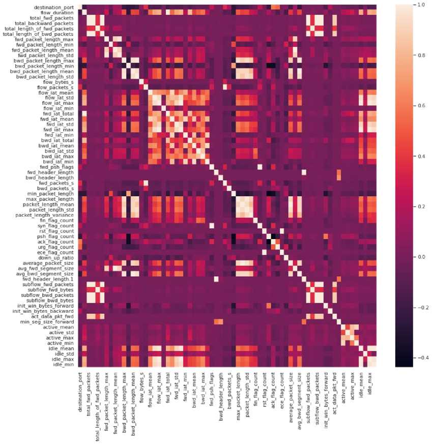
Fig.1. Heatmap of feature correlation

The “label” column was selected as the target and it was necessary to investigate the uniqueness of the values contained therein. A plot of the network activity was created, with 'Network activity' on the x-axis and 'Number of instances' on the y-axis This plot revealed that the dataset was highly skewed (shown in Figure 2).

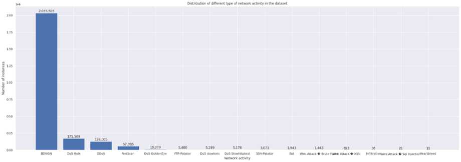
Fig.2. High skew of CICIDS 2017 dataset

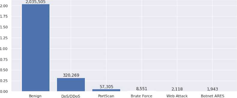
The attacks contained in the “label” column were thereafter regrouped as shown in Table 5 and displayed in Figure 3. However, the “infiltration” category was dropped due to small number of attack samples.

Table 5. Column regrouping for attacks in CICIDS 2017 dataset

GROUP	ATTACK	NUMBER OF SAMPLES
Benign	BENIGN	2035505
PortScan	PortScan	57305
DoS/DDoS	DDoS	320269
	DoS Hulk
	DoS GoldenEye
	DoS slowloris
	DoS Slowhttptest
	Heartbleed
Brute Force	FTP-Patator	8551
	SSH-Patator
Botnet ARES	Bot	1943
Web Attack	Web Attack Brute Force	2118
	Web Attack Sql Injection
	Web Attack XSS

Network activity

Fig.3. Reframed attack grouping

• 3.3.    Train and Test Data Split

  Since the CICIDS2017 dataset is not composed of a separate training data as well as test data (unlike datasets such as NSL-KDD), it is required for machine learning model development, that this dataset be separated into a training as well as a test section. In this work, the train test split tool from Sklearn library was used to achieve this. A twenty percent test to eighty percent training data split was implemented for developing both shallow learners and the deep

• 3.4.    Feature Selection and Engineering

  For the shallow learning algorithms, not all the features in the default CICIDS 2017 data were used to train. In order to obtain the features with the higher factor of importance, first of all, a test data of size 0.3 was selected and the Decision Tree classifier was used to train with a cross validation number of 10 and max_leaf_nodes=5 (chosen randomly). The optimal features were four namely Average Packet Size, Bwd Packet Length, Bwd Header Length and FIN Flag Count as displayed in Figure 4.

neural network. The default random process for data groups construction via the train test split function was adopted for the shallow learning classifiers. However, for the deep neural network, the split was stratified in order to ensure approximate similarity in ratio among the training as well as test dataset.

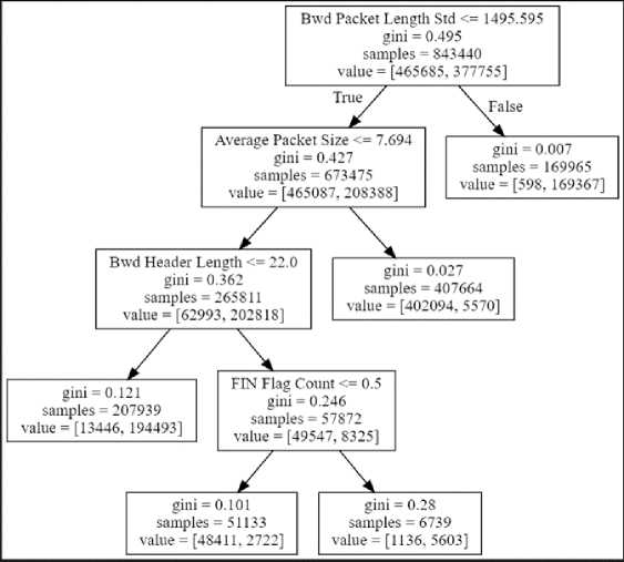
Fig.4. Feature importance with decision tree

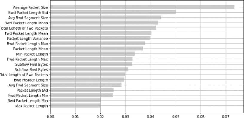
Table 6. Top twenty features from random forest classifier selection

S/N	FEATURE POSITION	WEIGHT	FEATURE NAME
1.	#51	0.073	Average Packet Size
2.	#12	0.050	Bwd Packet Length Std
3.	#53	0.044	Avg Bwd Segment Size
4.	#11	0.043	Bwd Packet Length Mean
5.	#3	0.042	Total Length of Fwd Packets
6.	#7	0.040	Fwd Packet Length Mean
7.	#41	0.040	Packet Length Variance
8.	#9	0.038	Bwd Packet Length Max
9.	#39	0.037	Packet Length Mean
10.	#37	0.034	Min Packet Length
11.	#5	0.033	Fwd Packet Length Max
12.	#61	0.033	Subflow Fwd Bytes
13.	#63	0.031	Subflow Bwd Bytes
14.	#4	0.030	Total Length of Bwd Packets
15.	#34	0.030	Bwd Header Length
16.	#52	0.029	Avg Fwd Segment Size
17.	#40	0.025	Packet Length Std
18.	#6	0.025	Fwd Packet Length Min
19.	#10	0.020	Bwd Packet Length Min
20.	#38	0.020	Max Packet Length

This was also verified using the SelectFromModel tool imported from the Sklearn.feature_selection library. The estimator=decision_tree argument was set and the sample dataset trained. Selecting a sfm. threshold of 0.0135135, four features met this threshold requirement namely Average Packet Size (0.4847593), Bwd Packet Length Std (0.3437284), Bwd Header Length (0.1521656) and FIN Flag Count (0.0193466) same as obtained in Figure 4. However, using only four features for attack classification could lead to bias. Hence instead of a single decision tree, a Random Forest approach for selecting optimal feature importance was thereafter adopted. The RandomForestClassifier was imported from the sklearn.ensemble library and the n_estimators=250, random_state=42 arguments were set. After achieving an accuracy score of 99% on the sample test data, the first twenty features used for clarification were adopted as shown in Table 6. With this method, a decision-forest is usually created when running the algorithm and each attribute is assigned a weight of relevance with respect to the decision tree in focus. At the end of the process, there is comparison and orderly arrangement of the feature importance weights such that, the overall important weight of the decision tree corresponds to the sum of the importance weights of the entire attributes. The distribution plot for the resulting top twenty most important features is further displayed in Figure 5.

Relative Importance

Fig.5. Distribution plot for top twenty features by random forest

For the deep learning model, undersampling via the RandomUnderSampler function as well as oversampling via the Synthetic Minority Oversampling Technique (SMOTE) were applied respectively on the data to mitigate the skew. The rationale for employing the undersampling technique was to reduce the number of samples in the majority classes (such as Benign, PortScan and DoS/DDoS). This could help provide some form of balance to the class distribution for the training data (shown in Figure 3). This could also result in less training time and computational requirements which are desired advantages while training deep learning models [32]. SMOTE was used for oversampling due to the added benefit of non-information loss since there is no removal of any sample. SMOTE further reduces the likelihood of overfitting because synthetic samples which are variant from original data samples are generated. The synthetic samples introduced thus improve the overall performance of the deep learning model [32].

• 3.5.    Model Building

By employing a Python package known as LazyPredict on a subset of the data , the five shallow machine learning classifiers adopted in this work were selected out of twenty-six considered. The LazyClassifier was employed with the argument, “verbose=1”. The classifiers were adopted based on their overall optimal F1-score and execution time with LazyPredict as displayed in Table 7 . LazyPredict package is used to build machine learning models with less coding thus saving computation power. It further provides insight into which models work better than others for a specific dataset without tuning any parameter [33]. It was adopted for obtaining the shallow classifiers due to relatively low computational cost.

Table 7. Performance of selected shallow learners with lazypredict package

Classifier	F1-Score (%)	Time Taken (secs.)
Decision Tree	97.66	0.0161
XGB	97.75	0.2496
MLP	55.94	0.0123
KNN	97.49	0.0460
Random Forest	97.58	0.2008

After training, the performances of the five classifiers in terms of Precision, Accuracy, F1-score and Recall were thereafter evaluated.

The developed deep learning (Deep Neural Network) model comprised six hidden dense layers, with Rectified Linear Activation Unit (ReLU) function to introduce non-linearity in the layers (where ReLU ( z ) = (0, z )). The first to sixth layer had 256, 128, 64, 32, 16 and 8 neurons respectively. The output layer was given a Softmax activation function. Softmax function described by Equation 1 inputs some vector element (x) of M real numbers, then it carries out normalization into an equivalent distribution of M probabilities.

S ( x ) i =

exi

z

M j=1

e

xi

For minimization process, SparseCategoricalCrossentropy was employed for loss function while developing the deep learning model, where Loss ( L_SCC E ) = — Z G_=iyjl°g ( У j ), and G = no. of classes , y j = actual probability and ^yj = predicted pwbability . Adam optimizer was adopted with a learning rate of 0.001 since it gives higher accuracy compared to higher or lower values. The deep neural network model was then configured with the following hyperparameters batch_size=32, epochs=5. These values were adopted because they produced optimal results with the model. The model was set to run for 5 epochs because beyond the 5^th epoch there were no further improvements in the model accuracy. The time for each epoch run is shown in Table 9.

4.    Performance Results and Associated Discussion

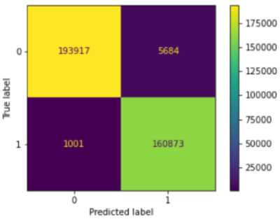
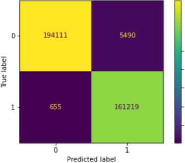
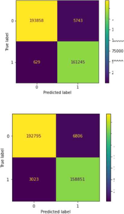
Figures 6 to 10 display the various confusion matrices for the Decision Tree, XGB, MLP, KNN and Random Forest classifiers respectively. Table 8 presents the result summary for the five shallow classifiers considered, while Table 9 displays the result summary for the deep neural network developed. Accuracy, Precision, Recall and F1-score were chosen as metrics to evaluate the shallow classifiers because they are values obtained directly from the various confusion matrices represented directly below. Figure 11 displays the accuracy versus epoch curve for the DNN while Figure 12 displays the loss versus epoch curve.

• Fig.6.    Decision tree confusion matrix

  

  - 175000

  I- 150000

  
  

• Fig.7.    XGB confusion matrix

  - 175000

  - 150000

  Ь 125000

  к юоооо

  
  
  

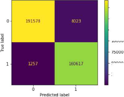
Fig.8. MLP confusion matrix

Fig.9. KNN confusion matrix

- 175000

к 150000

•150000

I-125000

ЮОООО

Fig.10. Random forest confusion matrix

Table 8. Result summary for shallow learning models

Classifier	Accuracy	Precision	Recall	F1-score	Time Taken (secs.)
Decision Tree	98.1%	98.0%	98.2%	98.1%	4.567
XGB	98.3%	98.18%	98.42%	98.28%	52.12
MLP	97.4%	97.29%	97.6%	97.4%	45.396
KNN	98.1%	98.0%	98.2%	98.1%	1344
Random Forest	97.3%	97.0%	97.2%	97.1%	3.95

Table 9. Training and validation results for deep learning model

EPOCH RUN	TIME	LOSS (TRAINING)	ACCURACY (TRAINING)	LOSS (VALIDATION)	ACCURACY (VALIDATION)
1	112 secs.	0.0614	97.68%	0.0211	99.01%
2	113 secs.	0.0320	98.85%	0.0334	98.95%
3	105 secs.	0.0260	99.18%	0.0181	99.48%
4	109 secs.	0.0224	99.36%	0.0127	99.71%
5	111 secs.	0.0202	99.41%	0.0182	99.53%

Fig.11. Deep learning accuracy

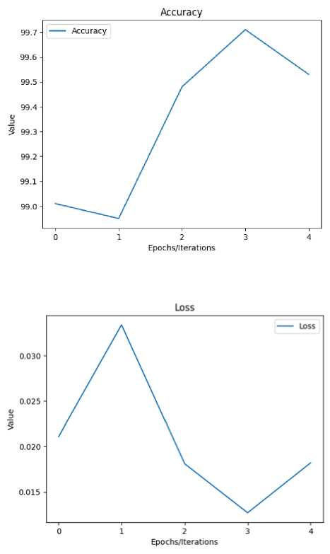
Fig.12. Deep learning loss

For the shallow learning classifiers, Decision Tree was chosen as a baseline model for comparing the performances of other shallow learning classifiers considered. As seen in Table 8, XGB presents the highest accuracy and F1-score, with 0.2% and 0.18% higher than the respective values for the baseline model (i.e., Decision Tree). However, it took the second highest execution time of 52.12 seconds, whereas Decision Tree took 4.567 seconds. From a classification performance perspective therefore, XGB performed higher than the baseline, but from a speed perspective it performed less than the baseline. MLP performed slightly less than the baseline model at classification, and performed considerably less in terms of speed. KNN performed exactly the same with Decision Tree during classification but was the slowest of all the shallow learning classifiers considered (taking 1344 seconds). Random Forest had a faster execution time than the baseline model, but presented accuracy of 0.8% and F1-score of 1% less than the baseline respectively. Summarily, of all the shallow learning classifiers considered, XGB performed best at classification but Random Forest performed best in terms of speed.

The deep neural network model displayed the best performance of all models considered, in terms of accuracy. As seen in Table 9 it presented a value of 99.71% at the 4th epoch. However, it presents a longer training time compared to shallow learning classifiers such as Decision Tree and Random Forest. This is however understandable in the light of deep learning models performing deeper levels of packet inspection to unravel the abstractions in the data.

5.    Conclusions

The burden of resolve in this work was the comparison of performance analysis between various shallow machine learning algorithms and a deep learning algorithm all on the pedestal of the combined CICIDS 2017 dataset. The CICIDS 2017 dataset was imported as a CSV file, pre-processed and the necessary feature selection and engineering carried out for the development of shallow as well as deep learning classifiers. Various performance metrices were used to evaluate the developed attack classification models. It was found that in terms of accuracy, the deep learning model outperformed all the shallow learning models considered. It was followed by XGB in terms of performance for attack classification. The deep learning model surpassed the accuracy of all models in considered literature, while XGB surpassed the accuracies of all ML models considered in [15,19-21]. However, in terms of processing time, some shallow learning classifier such as the base line Decision Tree and Random Forest had less processing time than both the deep learning model and XGB. The information provided by this study is to serve as guide for cybersecurity solutions developers who implement intrusion detection systems with the CICIDS 2017 dataset on which model to implement in developing necessary intrusion detection systems. Any adopted model from this study can then be interfaced with relevant application programming interface or web framework such as Hug, Flask, Falcon, and so on, for deployment in stationary or mobile devices in the production environment.

Acknowledgment

The authors hereby appreciate the Canadian Institute for Cybersecurity, at the University of New Brunswick, Canada for allowing the CICIDS 2017 dataset to be made public material.