Performance Analysis of Software Effort Estimation Models Using Neural Networks

Published Online August 2013 in MECS

Estimating software development effort remains a complex problem, and the one which continues to drawsignificant research attention. Software project managers usually estimate the software development effort, cost and duration in the early stages of a software life cycle in order to appropriately plan, monitor and control the allocated resources. Correctness in estimating the required software development effort plays a critical factor in the success of software project management Right amount of resource should be allocated to a project. If too much of resource is allocated to the project to is called as overestimation. If insufficient resource is allocated to the project is called underestimation. Software development activity involves lot of uncertainties the requirement will change, the developing platform will change, the developers capability to vary from one person to another lot of uncertainties are involved in the contributing factors which decides the effort required to develop the software. Hence soft computing frame work can be used that are good in handling the uncertainty. For good software estimation tool the estimated effort should be equal to the actual effort. Accurate estimation allows manager to allocate the resource to plan and coordinate all activities.

The large expenditures made by many companies for the development of software, even small increases in prediction accuracy are likely to be worthwhile. Underestimating costs can lead to accepting projects that do not provide enough returns or that overrun schedules, possibly with terrible consequences. Overestimating costs can lead to sound projects being rejected and can lead to gaps between one project ending and another starting This idle time can be expensive in competitive time-to-market industries. Either way, it is clear that more accurate estimates have considerable value to a corporation involved in software development. Once an estimation model has been derived it is vital that the limitations of the techniques used to develop and implement the model are understood in order to make sure that it is only used within its limitations.

Accurate Software cost estimation is always a difficult task. Estimation by experts, analogy-based estimation and soft computing methods are some of the effort estimation methods. In estimation by experts, the entire project is subdivided into small activities and with previous experience in effort estimation the developer of software estimate the effort depending on the type of task under consideration [1]. In analogy based estimation is a form of CBR. Cases are defined as abstractions of events that are limited in time and space [2].In soft computing based approach several technique like neural network fuzzy logic, genetic engineering are used either individually or combined as hybrid approaches to predict the effort [3].Complexity and uncertain behaviour of software projects are the main reasons for going toward the soft computing techniques

• [4] . Soft computing based approach play a prominent role because the ability of the soft computing frame work to learn from previous projects especially neural network is good in learning. Now a day’s estimation method using neural network is the interesting area for research compared to Theoretical estimation methods [5]. While considering the neural network lot of neural network architecture are available. Among which the most widely used method was Back propagation network. Elman network is a type of recurrent network that is equally as important as Back propagation algorithm. In our experiment both methods are used for estimating software development effort and their performance characteristics are analyzed.

The paper is organized as follows. Section 2 gives the detail about the related works and section 3 talks about the research methodology and the brief description about the Back propagation algorithm and ELMAN neural network. Section 4 gives detail about the dataset used. Section 5 gives detail about the experimentation, section 6 about evaluation criteria. Results and conclusion are given in section 7 and section 8 respectively.

• II.    Related Works

The use of Artificial Neural Networks to predict software development effort has focused mostly on the accuracy comparison of algorithmic models rather than on the suitability of the approach for building software effort prediction systems.Abbas Heiat [6] compares the prediction performance of multilayer perception and radial basis function neural networks to that of regression analysis. The results of the study indicate that when a combined third generation and fourth generation languages data set were used, the neural network produced improved performance over conventional regression analysis in terms of mean absolute percentage error Neural networks are often selected as tool for software effort prediction because of their capability to approximate any continuous function with arbitrary accuracy[7].Use of back propagation learning algorithms on a multilayer perceptron in order to predict development effort was described by Witting and Finnie[8,9]. The study of Karunanithi [10] reports the use of neural networks for predicting software reliability; including experiments with both feed forward and Jordon networks. The Albus multiplier perceptron in order to predict software effort was proposed by Samson [11]. They use Boehm’s COCOMO dataset. Srinivazan and Fisher [12] also exhibit the use of a neural network with a back propagation learning algorithm. But how the dataset was divided for training and validation purposes is not clearly mentioned. Iris febine et al[13] compares regression technique with artificial neural networks and found artificial neural network to be better than regression. Shift-invariant morphological system to solve the problem of software development cost estimation [14]. It consists of a hybrid morphological model, which is a linear combination between a morphological-rank operator and a Finite Impulse Response operator, referred to as morphological-rank-linear filter. Yan fu et al[15] adaptive ridge regression system can significantly improve the performance of regressions on multi-collinear datasets and produce more explainable results than machine learning methods.Finally in the last years; a abundant interest on the use of ANNs has grown. ANNs have been fruitfully applied to several problem domains. They can be used as predictive models because they are modeling techniques having the capability of modeling complex functions

• III.    Research Methodology:

Problem Statement: Understanding and calculation of models based on historical data are difficult due to inborn complex relationships between the related attributes, are unable to handle categorical data as well as lack of reasoning abilities. Besides, attributes and relationships used to estimate software development effort could change over time and differ for software development environments. In order to overcome to these problems, a neural network based model with accurate estimation can be used.

The COCOMO II model: The COCOMO model is a software cost estimation model based on regression. It was developed by Barry Bohem the father of software cost estimation in 1981. Among of all traditional cost prediction models. COCOMO model can be used to calculate the amount of effort and the time schedule for software projects. COCOMO 81 was a stable model on that time. One of the problems with using COCOMO 81 today is that it does not match the development environment of the late 1990’s. Therefore, in 1997 COCOMO II was published and was supposed to solve most of those problems. COCOMO II has three models also, but they are different from those of COCOMO 81. They are

• •    Application composition model-mostly suitable for projects built with modern GUI-builder tools. Based on new Object Points

• •    Early Design Model-To get rough estimates of a project's cost and duration before have determined its entire architecture. It uses a small set of new Cost Drivers and new estimating equations. Based on Unadjusted function Points or KSLOC

• •    Post-Architecture Model-The most detailed on the three, used after the overall architecture for the project has been designed. One could use function points or LOC as size estimates with this model. It involves the actual development and maintenance of a software product

COCOMO II describes 17 cost drivers that are used in the Post-Architecture model [16]. The cost drivers for

COCOMO II is rated on a scale from Very Low to Extra High in the same way as in COCOMO 81.

COCOMO II post architecture model is given as:

Effort =  ×

[size]B× ∏ Effort Multiplier^

where

В =1.01+0.01×

∑ Scale factor^j=i

A = Multiplicative constant

Size = Size of the software project measured in terms of KSLOC (thousands of source lines of code, function points or object points)

The selection of Scale Factors (SF) is based on the rationale that they are a significant source of exponential variation on a project’s effort or productivity variation. The standard numeric values of the cost drivers are given in Table 1.The cost drives and scale factors are given as input to the neural network with effort as the networks output. Two type of network used for analysis are discussed below.

What are neural network? Neural networks are a computational representation inspired by studies of the brain and nervous system in biological creatures. They are highly idealized mathematical models of how we understand the principle of these simple nervous systems. The basic characteristics of a neural network are (i)It consists of many simple processing units, called neurons, that perform a local computation on their input to produce an output. (ii). Many weighted neuron interconnections encode the knowledge of the network. Weight value is set according to the input output pair. (iii)The network has a leaning algorithm that lets it automatically develop internal representations. One of such algorithm is called levenberg-marquardt algorithm. (iv) Activation functions like sigmoid, linear activation function can be used. Two well-known classes suitable for prediction applications are feed forward networks and recurrent networks. In the main text of the article, we are concerned with feed-forward networks and a variant class of recurrent networks, called ELMAN networks. We selected these two model classes because we found them to be more accurate in reliability predictions than other network models

• 3.1    Back Propagation Network:

The back propagation learning algorithm is one of the most widely used method in neural network. The network associated with back-propagation learning algorithm is called as back propagation network. While training a network a set of input-output pair is provided the algorithm provides a procedure for changing the weight in BPN that helps to classify the input output pair correctly. Gradient descent method of weight updating is used [17].

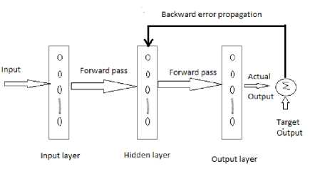
Fig. 1: Back propagation Network

The aim of the neural network is to train the network to achieve a balance between the net’s ability to respond and its ability to give reasonable responses to the input that is similar but not identical to the one that is used in training. Back propagation algorithm differs from the other algorithm by the method of weight calculation during learning. The drawback of Back propagation algorithm is that if the hidden layer increases the network become too complex

Procedure for Back propagation algorithm:

Let the input training vector x = (x₁,……., x_i,…….,x_n) and target output vector t = (t₁,…..,t_k,……t_m) the effort multiplier and scale factor can be given as the input x and the target effort is presented as t. α represents the learning rate parameter, v oj = bias on j^th hidden layer, w ok = bias on k^th hidden layer, z j hidden unit j, the net input to z j is

Zinj=voj + ∑ кх^ц and the output is zj=f(Zinj)

yk = output unit k. the net input to yk is yink=wok + ∑MZiWik and the output is

Y k =f(y ink )

• 3.2    Elman Network

  Elman Network was first proposed by Jeffrey L. Elman in 1990.Elman neural network is feed forward network with an input layer, a hidden layer, an output layer and a special layer called context layer. The output of each hidden neuron is copied into a specific neuron in the context layer. The value of the context neuron is used as an extra input signal for all the neurons in the hidden layer one time step later. In an Elman network, the weights from the hidden layer to

the context layer are set to one and are fixed because the values of the context neurons have to be copied exactly. Furthermore, the initial output weights of the context neurons are equal to half the output range of the other neurons in the network. The Elman network can be trained with gradient descent back propagation and optimization methods. A recurrent network is one in which there is a feedback from neuron’s output to its input. The input to the network is x1,x2,x3 xn and the output of the network is taken as y1,y2,y3---yn. The output of the hidden layer (h1, h2, h3--- hn) are fed back again to hidden layer neuron using context node (c1,c2,c3 cn). Unlike feed forward neural networks, Recurrent Neural Networks can use their internal memory to process arbitrary sequences of inputs. The output of each hidden neuron is copied into a specific neuron in the context layer.

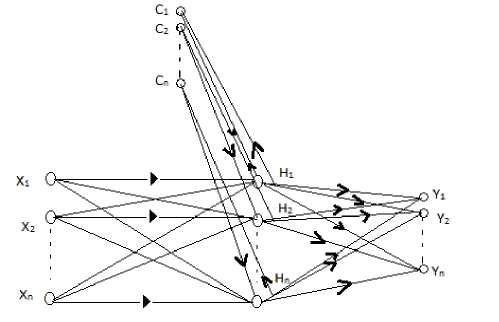
Fig. 2: ELMAN Network

TURN are used only in COCOMO 81 and some new attributes like RUSE, DOCU, PCON, SITE are introduced in COCOMO II.

Table 1: Effort Multipliers and their Range

Effort Multipliers		Range
Required software Reliability	RELY	0.82-1.26
Data base size	DATA	0.90-1.28
Product Complexity	CPLX	0.73-1.74
Developed for Reusability	RUSE	0.95-1.24
Documentation Match to Life- Cycle needs	DOCU	0.81-1.23
Execution Time Constraints	TIME	1.00-1.63
Main storage Constraint	STOR	1.00-1.46
Platform Volatility	PVOL	0.87-1.30
Analyst capability	ACAP	1.42-0.71
Programmer capability	PCAP	1.34-0.76
Personal continuity	PCON	1.29-0.81
Applications Experience	APEX	1.22-0.81
Platform Experience	PLEX	1.19-0.85
Language and Tool Experience	LTEX	1.20-0.84
Use of software tool	TOOL	1.17-0.78
Multisite Development	SITE	1.22-0.80
Required Development Schedule	SCED	1.43-1.00

The value of the context neuron is used as an extra input signal for all the neurons in the hidden layer one time step later. In an Elman network, the weights from the hidden layer to the context layer are set to one and are fixed because the values of the context neurons have to be copied exactly.

• IV.    Dataset Description

Dataset used for analysis and validation of the model can be got from historic projects of NASA. One set of dataset consists of 63 projects and other consists of 93 datasets. The datasets is of COCOMO II format. In our experiment 93 datasets are used for training and 63 data is used for testing.

The Dataset need for training as well as testing is available in and in . The dataset available is of COCOMO 81 format which is to be converted to COCOMO II by following the COCOMO II Model definition manual [18] and Rosetta stone [19] COCOMO 81 is converted to COCOMO II. COCOMO 81 is the earlier version developed by Barry Boehm in 1981 and COCOMO II is the next model developed by Barry Boehm in year 2000. Some of the attributes like

Every input as Effort multiplier has been tuned by following the COCOMO II model definition manual [18]. The scale factor and Effort multiplier and their range is given in Table I and II. One of such inputs RELY can be discussed below in Table III:

Table 2: Scale factors and their range

Scale Factor		Range
Precedentedness	PREC	0.00-6.20
Development Flexibility	FLEX	0.00-5.07
Architecture/Risk Resolution	RESL	0.00-7.07
Team Cohesion	TEAM	0.00-5.48
Process Maturity	PMAT	0.00-7.80

The Rating levels are fixed by the developer. If the failure of the software causes slight inconvenience and the corresponding rating level is very low, then the effort multiplier is fixed to be 0.82. In case of some software failure can easily be recoverable then the corresponding rating level is Nominal and rating level is fixed to be 1. If the failure of the software causes risk to human life the rating level given by the developer is very high then the effort multiplier is fixed to be 1.26

Table 3: Fixing Input attributes

RELY Descriptor	Rating Levels	Effort Multipliers
Slight Inconvenience	Very Low	0.82
Low, easily recoverable loss	Low	0.92
Moderate, easily, recoverable loss	Nominal	1
High financial, loss	High	1.1
Risk to Human life	Very High	1.26

• V.    Experimentation

Neural Network Uses two set of datasets One set of dataset consists of 63 projects and other consists of 93 datasets both are from the historic projects of NASA. Here we use 93 projects for training the network and 63 projects for testing. The simulation is done in MATLAB 10b environment. In back propagation and Elman network the weight and bias are randomly fixed so each time there is a possibility of getting different result to avoid this problem the whole network is made to run for 50 iteration and their errors are summed up.

The network designed uses only one hidden layer and that hidden layer has eight neurons and output layer has one neuron. The hidden layer uses sigmoid transfer function. And output layer uses linear transfer function. The above consideration is used for both Back propagation as well as ELMAN network for uniformity. Input fed to the neural network is normalized using Premnmx and the output is DE normalized using postmnmx. Premnmx normalizes the value between (-1 to 1)

• VI.    Evaluation Criteria

For evaluating the different software effort estimation models, the most widely accepted evaluation criteria are the mean magnitude of relative error (MMRE), Probability of a project having relative error less than 0.25, Root mean square of error, Mean and standard deviation of error.

The magnitude of relative error (MRE) is defined as follows

| actual effort,—predicted effort; |

1              actual effort;

The MRE value is calculated for each observation I whose effort is predicted. The aggregation of MRE over multiple observations (N) can be achieved through the mean MMRE as follows

MMRE = ∑ У MRE,                  (2)

PRED (25)= MRE<0 ^. 25                         (3)

Consider Y is the neural network output and T is the desired target. Then Root mean square error (RMSE) can be given by

RMSE = √( Y - T )²

Error can be calculated by the difference between Y and T then mean and standard deviation is calculated by calculating the mean and standard deviation of the error

ERROR=(Y-T)

• VII.    Results

Comparison results of BPN and ELMAN for training is given below in Table. IV. And the comparison results of BPN and ELMAN for testing is given in Table. V. A model which gives lower MMRE is better than the model which gives higher MMRE. A model which gives high PRED (25) is better than the model which gives lower PRED (25). Similarly the model which gives lower RMSE is better than the model which gives higher RMSE. The model which mean and standard deviation is closer to zero is better than the models which gives mean and standard deviation far away from zero.

Table 4: Results of Training for BPN

Performance Measures	BPN
	MIN	MAX	MEAN
MMRE	0.0371	0.2105	0.0928
PRED(25)	67.7419	98.9247	91.8065
RMSE	0.3422	1.383	0.6774
MEAN	-0.3975	0.3167	7.75E-04
Std.Dev	0.3418	1.3535	6.72E-01

Table 5: Results of Training for ELMAN

Performance Measures	ELMAN
	MIN	MAX	MEAN
MMRE	0.0357	0.208	0.0936
PRED(25)	69.8925	98.9247	92.3656
RMSE	0.366	1.2544	0.6748
MEAN	-0.3207	0.3422	0.0083
Std.Dev	0.3678	1.241	0.666

Table 6: Results of Testing BPN

Performance Measures	BPN
	MIN	MAX	MEAN
MMRE	0.1712	3.7931	0.3846
PRED(25)	30.1587	82.5397	63.5873
RMSE	0.8285	2.2076	1.3142
MEAN	-1.6898	0.8806	-0.1141
Std.Dev	0.7306	1.8707	1.2233

Table 7: Results of Testing ELMAN

Performance Measures	ELMAN
	MIN	MAX	MEAN
MMRE	0.1678	3.4354	0.4467
PRED(25)	42.8571	79.3651	60.4444
RMSE	0.8566	3.5265	1.4
MEAN	-1.4708	0.8159	-0.2003
Std.Dev	0.8312	3.2309	1.314

The results of BPN and ELMAN for testing are given in table VI and VII. From above result it is confirmed that BPN has lower MMRE, RMSE higher PRED (25) and mean and standard deviation closer to zero. Fig 3 represents the Comparison of MMRE for BPN and ELMAN Fig 4 represents the Comparison of RMSE for BPN and ELMAN

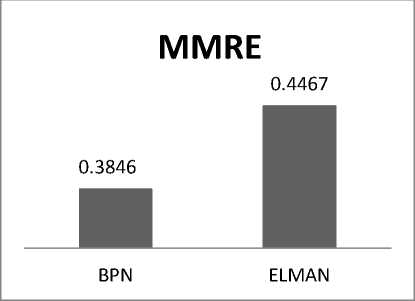
Fig. 3: Comparison of MMRE for BPN and ELMAN

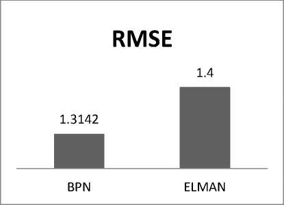
Fig. 4: Comparison of RMSE for BPN and ELMAN

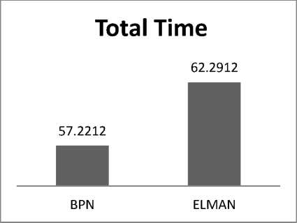
Fig. 5: Comparison of time taken for BPN and ELMAN network

BPN completes 50 iteration in 57.2 sec compared to 62.2 sec of ELMAN network. Thus BPN has lower computation time than ELMAN network

• VIII.    Conclusion

Most important thing in software effort prediction is its closeness to actual effort. we have analyzed the performance of both using historic dataset of NASA From the above results it is confirmed that BPN is best suited for software cost estimation compared to ELMAN network. BPN produces accurate estimate with less time compared to ELMAN network. The work can be extended to hybrid computing techniques like Fuzzy based BPN and Fuzzy based ELMAN. Further it can be extended to new and advanced learning algorithm like ELM, MRAN, Meta cognitive neural network etc. Results can be further validated using different type of dataset or simulated dataset. In simulated dataset the relation between the input and output is known.