Performance Evaluation of Modified DBLA Using Dark Channel Prior & CLAHE

Producing digital images with good brightness/ contrast and detail is a strong requirement in several areas like visualization, remote sensing, biomedical image examination, error recognition. The primary constraint for almost all vision and image processing task is produce natural images and transforming the image such as to enhance the visual information. Image enhancement is used to accentuate and sharpen image features for demonstrate and analysis. Image enhancement is the practice of applying these techniques to assist the improvement of a result to a computer imaging crisis. These methods are function exact and developed experimentally. These kinds of methods include point operation, where each pixel is customized according to a fastidious equation that is independent on other pixel values; mask operations, where each pixel is customized according to the values of the pixel’s neighbors; or global operations, where all the pixels values in the image are taken into concern. Spatial domain processing methods take account of all three types, but frequency domain operations, by character of the frequency transforms, are universal operations. Frequency domain operations are able to develop into mask operations, based only on a local neighbourhood, by performing the transform on small image blocks rather than whole image. For easy visual task enhancement is used as a preprocessing step in some computer vision applications, for example, to enhance the edges of an object or it is also used in applications where human screening of an image is essential before additional processing. It is also applicable for post processing process to generate a visually desirable image. In short image enhancement is a method to make images look better visually. For the contrast enhancement method, CLAHE method is used that to avoid the problems of HE and AHE that is amplification of the noise. This paper represents the integrated approach to overcome the problems of existing techniques. In this perform a contrast enhancement by using the integrated approach using dominant brightness level analysis, contrast limited adaptive histogram equalization and dark channel prior algorithm.

• II.    Contrast Limited Adaptive Histogram Equalization

Contrast limited adaptive histogram equalization prevent the amplification by using contrast limiting. The contrast limiting procedure has to be applied for each neighborhood from which a transformation function is derived in contrast limiting adaptive histogram equalization. CLAHE does not operates on entire image, it is applicable for small regions that known as tiles. Contrast of small region (tiles) is enhanced. After matching histogram of the output region is then combined by using bilinear interpolation to abolish artificially induced boundaries. The contrast of homogeneous areas can be limited because it can reduce the amplification of noise that may occur in the image. CLAHE was basically introduced for medical imaging and it was successful to enhance the low contrast images such as portal films.

In this method no prior weather information is required to advance the quality of the image. In this the captured image is converted from RGB (red, green, and blue) colour space to the HIS (hue, saturation and intensity). This conversion is done because HIS colour space senses the colour same as the human eye. The HIS color model defines every color with hue, saturation and intensity components. After the conversion from RGB to HIS a relative region is set and then CLAHE method applies histogram equalization to a background region. Each pixel in the original image is in the center of background region. The original histogram is clipped and the clipped pixels are redistributed to each gray level. The new histogram is different with ordinary histogram, because pixel intensity is limited to a user-selectable maximum. First of all the average number of pixels are calculated according to the equation:

_ ⁿCR-XP ^{× n}cr-yp

N 14 arg

Ngray

Where ^avg an average number of pixels are, Ngray is number of gray pixels in background region, Ncr-xp is number of pixels in x dimension of background region, Ncr-yp and is number of pixels in y dimension of background region. The actual clip limit can be calculated as:

Ncl ^{=     ×} Navg

Where N_Cl is actual clip limit? The original histogram is clipped and the clipped pixels are redistributed to each gray- level.

A. CLAHE on RGB color model

RGB color space describes colors in terms of the amount of red ( R ), green ( G ) and blue ( B ) present. It uses additive color mixing, because it depicts that which type of light require to be emitted to create a given color. Light is added to create form from out of the darkness.

(a)

The value of R , G , and B components is the sum of the respective sensitivity functions and the incoming light.

R =∫Z5(Y)R(Y) dy(3)

G =∫Z5(Y)G(Y) dy(3)

В =∫Z5(Y)В(Y) dy(5)

where S(γ) is the light spectrum, R(γ), G(γ), B(γ) are the sensitivity functions for the R, G and B sensors respectively. In RGB color space, CLAHE can be applied on all the three components individually. The result of full-color RGB can be obtained by combining the individual components.

• III.    Dark Channel Prior

Dark channel prior is a statistics of outdoor image haze removal. It is based on the fact that the local patches in the haze free images whose intensity is very low in at least one color channel. This information is used by dark channel prior method to improve the quality of image. From these pixels whose intensity is low the thickness of the haze can be estimated and the high quality haze free image can be recovered. High quality depth map of the image can also be obtained in this method [2]. The dark channel prior is based on the observation on fog-free outdoor images that there is at least one color channel having very low intensity at some pixels. For an image J we define dark channel as:

jdark ⁽ X ) = min ce { r g b } (min YC Ω( x ) ( ( У ))         (6)

Where J^c a color channel of J and Ω (x) is a local patch centered at x. If J is a fog-free outdoor image then excluding the sky area, the intensity of jdark is low that mean approximately zero. We call jdark the dark channel of J. Due to the air light; a foggy image is brighter than its fog-free version in where the transmission t is low.

So the dark channel of the foggy image will have higher intensity in regions with denser fog. Thickness of the fog is a rough estimate of the intensity of the dark channel.

(b)

Fig. 1. shows the effect of CLAHE on RGB color model (a) Input image (b) CLAHE on RGB

• IV.    Dominant Brightness Level Analysis

As increasing demand for enhancing remote sensing images, presented histogram-based contrast enhancement methods notable to conserve edge details and demonstrate saturation artifacts in low and high intensity regions. If do not consider spatially varying intensity distributions, in the same way contrast-enhanced images may have intensity distortion and lose image details in some regions[1].

For overcoming these problems, decompose the input image into four different layers of single dominant brightness levels. Perform the DWT on the input remote sensing image and then estimate the dominant brightness level using the log average luminance in the LL sub band, for this low frequency components used. The low-intensity layer has the dominant brightness lower than the pre specified low bound.

(a)

(b)

Fig. 2. shows the results of dominant brightness level analysis (a) Input image (b) Dominant brightness level analysis image

• V.    Gaps in Survey

Following are the major disadvantages that are found in the related work of image enhancement techniques .

• 1.    The survey has found that the most existing techniques are based upon the transform domain methods, which may introduce the color artifacts.

• 2.    Transform domain method may reduce the intensity of the input remote sensing image.

• 3.    The use of dark channel and CLAHE in algorithm ignored by many researchers to reduce the problem of poor brightness which will be presented in the output image due to dominant level.

• VI.    Problem Definition

Image enhancement is one of the most popular algorithms used in vision applications for improving the visibility of the digital images. Recently much work is done in the field of remote sensing images to improve the visibility for improving their accuracy for further applications. Many algorithms have been proposed so far for enhancing the remote sensing images. It has been found that the most of the existing researchers have neglected many issues; i.e. no technique is accurate for different kind of circumstances. The existing methods have neglected the use of Contrast limited adaptive histogram equalization (CLAHE) to reduce the problem of poor brightness which will be presented in the image due to poor weather conditions. It is also found that the color artifacts which will be presented in the output image due to the transform domain methods; also neglected by the most of the researchers. So the present research work will use dark channel prior as the post processing function to enhance the results further.

The high intensity layer is resolute in the similar manner with the pre specified high bound, and the middle-intensity layer has the dominant brightness in between low and high bounds [1].

Since high-intensity values are dominant in the bright region, and similarly for low –intensity values, the dominant brightness at the position ( x, y ) is computed as:

D ⁽x,y) = exp (-^(xy^sUogL(x, y) + e) (7)

Where S represents a rectangular region encompassing ( x, y ), L ( x, y ) represents the pixel intensity at ( x, y ), NL represents the total number of pixels in S , and ε represents a satisfactorily small constant that prevents the log function from diverging to negative infinity. The low-intensity layer, high intensity layer and middle intensity layer has the dominant brightness level determined in the similar manner with pre specified low, high and middle bounds respectively. The normalized dominant brightness varies from zero to one, and it is practical range lies between 0.5 and 0.6 in most different images. For safely including the practical range of dominant brightness, we prefer 0.4 and 0.7 for the low and high bounds.

• VII.    Research Methodology and Experimental Set

UP

In order to implement the proposed algorithm, design and implementation has been done in MATLAB using image processing toolbox. In order to do cross validation we have also implemented the enhanced DCT based image fusion using nonlinear enhancement. The developed approach is compared against some well-known image fusion techniques available in literature. After these comparisons, we are comparing proposed approach against DCT using some performance metrics. Result shows that our proposed approach gives better results than the existing techniques.

To attain the objective, step-by-step methodology is used in this dissertation. Sub sequent are different steps which are used to accomplish this work. Following are the various steps used to accomplish the objectives of the dissertation.

Proposed algorithm

Step 1: Input images: select an input image. This image may be satellite image, foggy image, roadside image, natural image.

Step 2: Discrete wavelet transform: Now perform the DWT is a wavelet transform for which the wavelets are discretely sampled. Discrete wavelet transform captures both frequency and location information. Wavelet used for feature extraction, denoising, compression, face recognition, image super resolution.

Step3: Dominant brightness level analysis: This analysis is done to remove the problem of intensity distortion and lose image details due to contrast enhancement and divide image based on dominant brightness level analysis is into three intensity (low, middle, high).

Step4: adaptive intensity transfer function: then apply adaptive intensity transfer function on each layer and do boundary smoothing after smoothing weighting map estimation method applied on it.

Step5: contrast limited adaptive histogram equalization: then this technique is apply to prevent the limiting amplification and this also applicable for limiting the amplification of noise.

Step 6: inverse discrete wavelet transform: this technique is applied to reform the data.

Step 7: Dark channel prior: Basically this technique used for haze removal and improve the quality of image.

Step 8: final: Results has been shown in the form of contrast enhanced image.

(c)

(d)

• VIII.    Experimental Results

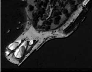
Fig 3 has shown the input images for experimental analysis. The overall objective is to combine relevant information from multiple images that is more informative and suitable for both visual perception and further computer processing.

(e)

(f)

(a)

(b)

(g)

Fig. 3. represents the final results proposed methodology (a) Input image (b) Dominant brightness level analysis image (c) Depth map (d) Transmission map (e) (f) CLAHE on RGB color model image (g) final image

• IX.    Performance Analysis

This section shows the results between existing and proposed techniques. Some well-known image performance parameters for digital images have been selected to prove that the performance of the proposed algorithm is quite better than the existing methods.

• A.    Mean square error

One understandable mode of measuring this correspondence is to calculate an error signal by subtracting the test signal from the reference, and then computing the average energy of the error signal. The mean-squared-error (MSE) is the simplest, and the most widely used, full-reference image quality measurement. This metric is frequently used in signal processing and is defined as follows:

MSE = ^E“ _г ^ ! (x( i,j ) - у ( i,j ))² (8)

Where x( i. j ) represents the original (reference) image and y( i, j ) represents the distorted (modified) image and i and j are the pixel position of the M×N image. MSE is zero when x( i, j ) = (i, j) .

Table 1. Mean square error

Image	DBL	RGB	PROPOSED
1.	338	667	213
2.	428	635	339
3.	296	948	189
4.	388	267	54
5.	119	229	29
6.	372	105	38
7.	355	442	71
8.	478	968	404
9.	168	510	84
10.	607	989	88
11.	268	636	165
12.	356	1017	239
13.	237	559	56
14.	184	184	87
15.	549	692	470

Comparative analysis of mean square error in Figure represent as:

Figure 1 has explained that quantized analysis of the mean square error. As mean square error need to be reduced therefore the proposed algorithm is showing the better results than the available methods as mean square error is less in every case.

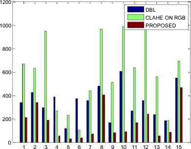
Fig. 1. Analysis of mean square error

• B.    Peak signal to noise ratio

Larger SNR and PSNR indicate a smaller difference between the original (without noise) and reconstructed image. This is the most widely used objective image quality/ distortion measure. The main advantage of this measure is ease of computation but it does not reflect perceptual quality. An important property of PSNR is that a slight spatial shift of an image can cause a large numerical distortion but no visual distortion and conversely a small average distortion can result in a damaging visual artifact, if all the error is concentrated in a small important region. This metric neglects global and composite error PSNR is calculated using Equation:

PSN8 = 20 log „ (^ d6               (9)

Comparative analysis of peak to signal ration in Figure represent as:

Table 2. Peak to signal ratio

Image	DBL	RGB	PROPOSED
1.	22.8416	19.8895	24.8470
2.	21.8164	20.1031	22.1211
3.	23.4179	18.3627	25.3662
4.	22.2425	23.8657	30.8069
5.	27.3753	24.5324	33.5068
6.	22.4254	27.9189	32.3330
7.	22.6285	21.6766	29.6182
8.	21.3365	18.2721	22.0670
9.	25.8777	21.0551	28.8880
10.	20.2989	18.1788	28.6860
11.	23.8495	20.0962	25.9560
12.	22.6163	18.0576	24.3468
13.	24.3833	20.6567	30.6489
14.	25.4826	25.4826	28.7356
15.	20.7351	19.7297	21.4098

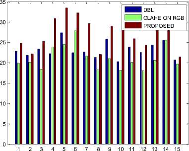
Fig. 2. Analysis of peak to signal ratio

Figure 2 is showing the comparative analysis of the Peak Signal to Noise Ratio (PSNR). As PSNR need to be maximized; so the main goal is to increase the PSNR as much as possible. Figure2 has clearly shown that the PSNR is maximum in the case of the DBL technique therefore it is providing better results than the available methods.

• C.    Root mean square error

The root mean square error is a normally used to calculate of the difference between values predicted by a model and values actually observed from the surroundings that is being modeled. These individual differences are also called residuals, and the RMSE serves to total them into a single measure of analytical power.

Table 3. Root mean square error

Image	DBL	RGB	PROPOSED
1.	18.3848	25.8263	14.5945
2.	20.6882	25.1992	19.9750
3.	17.2047	30.7896	13.7477
4.	19.6977	16.3401	7.3485
5.	10.9087	15.1327	5.5852
6.	19.2873	10.2470	6.1644
7.	18.8414	21.0238	8.4261
8.	21.8632	31.1127	20.0998
9.	12.9615	22.5832	9.1652
10.	24.6374	31.4484	9.3808
11.	16.3767	25.2190	12.8452
12.	18.8680	31.8904	15.4596
13.	15.3948	23.6432	7.4833
14.	13.5647	13.5647	9.3274
15.	23.4307	26.3059	21.6795

The RMSE of a model total with respect to the estimated variable X_{mode l} is defined as the square root of the mean squared error:

^Lik, Ss .-XmodeI .)²

R MSE = •—--^----- ^,^-

\       n

Where X_obs is observed values and X_model is modeled values at time/place i. As RMSE need to be minimized; so the main goal is to decrease the RMSE as much as possible.

Comparative analysis of root mean square error in Figure represent as below:

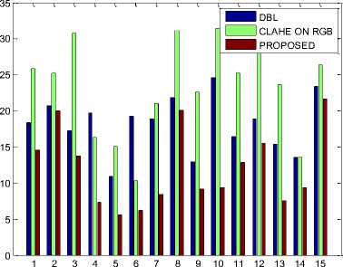
Fig. 3. Analysis of root mean square error

Figure 3 is showing the comparative analysis of the root mean square error (RMSE). As RMSE need to be minimized; so the main goal is to decrease the RMSE as much as possible. This is clearly shown that the RMSE is less in dominant brightness level.

• D.    Bit error rate

Bit error rate need to be minimized. Main goal is to decrease the BER as much as possible.

Table 4. Bit error rate

Image	DBL	HSV	RGB	PROPOSED
1.	0.0438	0.1426	0.0503	0.0402
2.	0.0458	0.0830	0.0497	0.0452
3.	0.0427	0.1316	0.0545	0.0394
4.	0.0450	0.3440	0.0419	0.0325
5.	0.0365	0.1175	0.0408	0.0298
6.	0.0446	0.3438	0.0358	0.0309
7.	0.0442	0.2779	0.0461	0.0338
8.	0.0469	0.1117	0.0547	0.0453
9.	0.0386	0.1137	0.0475	0.0346
10.	0.0493	0.964	0.0550	0.0349
11.	0.0419	0.1284	0.0498	0.0385
12.	0.0442	0.1382	0.0554	0.0411
13.	0.0410	0.1799	0.0484	0.0326
14.	0.0392	0.1201	0.0392	0.0348
15.	0.0482	0.1175	0.0507	0.0467

Comparative analysis of Bit error rate in Figure represent as:

Comparative analysis of root mean square error in Figure represent as below:

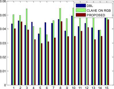
Fig. 4. Analysis of Bit error rate

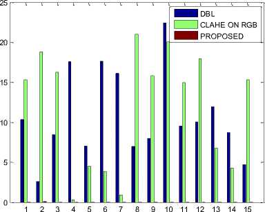
Fig. 5. Analysis of Average difference evaluation

Figure 4 is showing the comparative analysis of the BIT ERROR RATE (BER). As BER need to be minimized; so the main goal is to decrease the BER as much as possible. It has clearly shown that the BER minimum.

• E.    Average Difference Evaluation

Average difference is simply difference between the reference signal and test image. It is given by the equation.

AD =^Г= i^= i (x( iJ )-y( ij )) (11)

As average difference needs to be minimized; so the main objective is to reduce the average difference as much as possible.

Figure 5 is showing the comparative analysis of the AVERAGE DIFFERENCE EVALUTION (AD). As AD needs to be minimized; so the main goal is to decrease the AD as much as possible. It has clearly shown that the AD minimum.

F. Structural content

SC is also correlation based measure and measures the similarity between two images. Structural content is given by the equation

^=(((Ua^ ² ^^(xd.i)?

As SC needs to be close to 1, therefore proposed algorithm is showing better results than the available methods as SC is close to 1 in every case.

Table 5. Average Difference Evaluation

Image	DBL	RGB	PROPOSED
1.	10.3749	15.3312	0.0040
2.	2.6179	18.8196	0.0876
3.	8.4279	16.2675	0.0355
4.	17.5739	0.3007	0.0311
5.	7.0750	4.4720	0.0013
6.	17.6257	3.8261	0.0068
7.	16.1110	0.9463	0.0157
8.	6.9796	20.9881	0.0131
9.	7.9898	15.7940	0.0072
10.	22.3706	20.0926	0.0547
11.	9.5602	14.9370	0.0158
12.	10.0481	17.9571	0.0026
13.	11.9774	6.7968	0.0024
14.	8.7471	4.2851	0.0054
15.	4.7304	15.3147	0.0109

Table 6. Structural content

Image	DBL	RGB	PROPOSED
1.	0.8367	0.7276	1.0102
2.	0.8866	0.5731	1.0559
3.	0.8357	0.7534	1.0099
4.	0.8273	1.0181	1.0014
5.	0.9603	0.9603	1.0016
6.	0.8298	1.0364	1.0007
7.	0.8270	1.0008	1.0017
8.	0.8278	1.2212	1.0285
9.	0.8338	0.7448	1.0081
10.	0.8276	1.1372	1.0018
11.	0.8354	0.7287	1.0095
12.	0.8374	0.6948	1.0109
13.	0.8283	1.0623	1.0018
14.	0.8321	0.9018	1.0059
15.	0.8558	0.7779	1.0243

Comparative analysis of structural content in Figure represent as below:

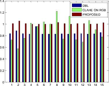
Fig. 6. Analysis of Structural content evaluation

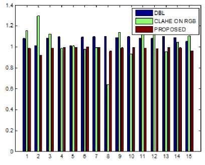
Fig. 7. Analysis of normalized cross-correlation evaluation

Figure 6 is showing the comparative analysis of the STRUCTURAL CONTENT (SC). As SC needs to be one; so the main goal is to maintain the SC as much as possible to one. It has clearly shown that the SC one.

G. Normalized cross correlation

V К — -- ~-------T—

Sg i S ?= 1И ,n)

Table 7. Normalized cross correlation evaluation

Image	DBL	RGB	PROPOSED
1.	1.0846	1.1616	0.9867
2.	1.0117	1.2950	0.9248
3.	1.0853	1.1221	0.9868
4.	1.0986	0.9871	0.9985
5.	1.0082	1.0082	0.9976
6.	1.0960	0.9809	0.9991
7.	1.0991	0.9919	0.9979
8.	1.0978	0.6416	0.9619
9.	1.0899	1.1417	0.9911
10.	1.0983	0.9301	0.9983
11.	1.0862	1.1570	0.9877
12.	1.0827	1.1786	0.9850
13.	1.0971	0.9553	0.9975
14.	1.0913	1.0448	0.9925
15.	1.0545	1.1053	0.9627

As NCC needs to be close to 1, therefore proposed algorithm is showing better results than the available methods as NCC is close to 1 in every case.

Comparative analysis of normalized cross-correlation in Figure represent as below:

Figure 7 is showing the comparative analysis of the normalized cross-correlation (NCC). As NCC needs to be close to one; so the main goal is to maintain NCC as much as possible to close to one. It has clearly shown that the NCC is more close to one.

• X.    Conclusion

Dominant brightness level analysis has been used to overcome the problems of intensity distortion and lose image details in some regions of contrast enhanced images without considering the spatially varying intensity distributions. For overcoming these problems, decompose the input image into multiple layers of single dominant brightness levels. To use the low-frequency luminance components, perform the DWT on the input remote sensing image and then estimate the dominant brightness level using the log average luminance in the LL sub band. The low-intensity layer has the dominant brightness lower than the pre specified low bound. The high intensity layer is determined in the similar manner with the pre specified high bound, and the middleintensity layer has the dominant brightness in between low and high bounds. The survey has found that the most existing techniques are based upon the transform domain methods, which may introduce the color artifacts. Transform domain method may reduce the intensity of the input remote sensing image. The use of dark channel and CLAHE in algorithm is ignored by many researchers to reduce the problem of poor brightness which will be presented in the output image due to dominant level. The proposed technique has modified the DBLA using CLAHE and dark channel prior. The modified DBLA has the potential to overcome the limitations of the earlier work. The proposed technique has been designed and implemented in MATLAB using image processing toolbox. The comparison among CLAHE, DBLA and proposed has shown the significant improvement of the proposed technique.