Performance of Data Replication Algorithm in Local and Global Networks under Different Buffering Conditions

Published Online August 2015 in MECS

Now a days, users in every countries is interested in online applications. Therefore the demand for higher bandwidth has increased tremendously in past one decade and it is expected to grow exponentially. The online users not only they do chatting but also downloads movies, audio and gaming application etc.. The huge demand of the bandwidth can’t be catered to using the electronic technology, due to the speed limitations of electronic devices [1]. However, optical fiber technology has the potential to support very high data rate with low loss and it also provide very large bandwidth to the users. In Optical switching two paradigm optical packet switching (OPS) and optical burst switching (OBS) are studied [12]. Optical packet switching works on the principle of connection less networking where packets are transferred form a node to another.

The generic layout of the OPS network is shown in Fig. 1. Here, the data inside the network cloud is optical, while outside the cloud is electronic in nature. The edge nodes have the capability of E/o and O/E conversion. In this work we only concentrate on the data movement inside the cloud in an OPS network .

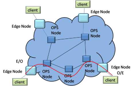
Fig. 1. Schematic of generic OPS network

However, OBS is a connection oriented switching techniques analogous to circuit switching where a path is first established then data follows the same path. In OBS the length of the burst is not fixed, and ideally it can vary from 2 packets lengths to some millions of packets. It must be remembered that the in OPS/OBS, a packet contain large data therefore it should not be lost. To avoid such loss, provisions are made in OPS and OBS. The loss of data may happen if two or more data’s try to occupy the same path in a single time slot and well referred as contention. For the contention resolution three solutions are proposed [3]:

• 1.    Wavelength conversion

• 2.    Buffering and

• 3.    Defection routing

Thus if contention can be resoled efficiently then the burst loss probability can be decreased with reasonable amount of delay. In this paper, for the contention resolution buffering of packets/bursts is considered. At the contending nodes, buffering can be employed in three ways:

• A.    Input Buffering

In input buffering scheme (Fig. 2), a separate buffer is placed at the each input of the switch and each arriving packets momentarily enter to buffering unit. If buffer is vacant, output port is free and in the other buffers (buffer available at other inputs) there is no packet for that particular output, then arriving packet will be forwarded to the appropriate output and if buffer is not empty then it will be placed in the buffer and will leave the buffer such that FIFO (First in First output) can be maintained for each output ports. In the input queuing head on blocking occurs and maximum possible throughput is only 0.586 [4].

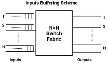
Fig. 2. Schematic of the input buffering scheme

• B.    Output Buffering

In output buffering scheme (Fig. 3), a separate buffer is placed at the each output port of the switch and arriving packets are transferred to appropriate output port and will be processed such that FIFO can be maintained. In the output queuing structure no internal blocking occurs. Therefore large throughput is achievable.

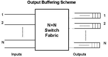
Fig. 3. Schematic of the output buffering scheme

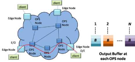
Fig. 5. Schematic of OPS network with output buffer at each node

In this paper we will only consider shared and output buffering of the contending information. Schematic of OPS network with output buffer at each node is shown in Fig. 5. Here, at each node with ‘ N’ input and output links a maximum of ‘ BN’ contending packets and for each output ‘ B’ packets can be stored separately. In figure 6, schematic of OPS network with shared buffer at each node is shown. Here, at each node with ‘ N’ input and output links can store a maximum of ‘ B’ contending packets can be stored in shared manner.

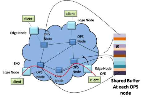
Fig. 6. Schematic of OPS network with shared buffer at each node

• C.    Shared Buffering

The above discussed input/output buffering schemes are not cost efficient because at each port separate buffer is required. Therefore hardware complexity is very large. In the shared buffering scheme (Fig. 4) packets for all the outputs are stored in the common shared buffer. Therefore hardware complexity is less and still higher throughput is achievable.

N

Shared Buffering Scheme

м

(N+M)x(N+M)

Switch Fabric

Inputs

Outputs

Fig. 4. Schematic of the shared buffering scheme

• D.    Data Replication

The communication means sending of information form a place to another. This communication can be one way, or two ways where from receiving end some data has to be fetched. The fetching of data form location to another is known as data replication. In general, replication is the process of copying and maintaining database objects, such as tables, in multiple databases that make up a distributed database system [5]. Changes applied at one site are captured and stored locally before being forwarded and applied at each of the remote locations. Replication uses distributed database technology to share data between multiple sites, but a replicated database and a distributed database are not the same. In a distributed database, data is available at many locations, but a particular table resides at only one location. Some of the most common reasons for using replication are described as follows:

• 1.    Replication provides fast, local access to shared data because it balances activity over multiple sites [5].

• 2.    Some users can access one server while other users access different servers, thereby reducing the load at all servers.

• 3.    Also, users can access data from the replication site that has the lowest access cost, which is typically the site that is geographically closest to them.

In past database replication was a rare event, but now it is very frequent. For example a multinational company, can have many office all over the world, and the database consistency is an important issues for maintaining stocks etc.. In this environment which generally changes with time, the location of the data can have a significant impact on application response time and availability [510]. In centralized approach only one copy of the database is managed. This approach is simple since contradicting views among replicas are not possible. However, the centralized replication approach suffers from two major drawbacks:

• •    high server load or high communication latency for remote clients.

• •    Sometime server may not be available due to the down time or lack of connectivity. Clients in portions of the network that are temporarily disconnected from the server cannot be serviced.

The server load and server downtime problems can be addressed by replicating the database servers to form a cluster of peer servers that coordinate updates. However, scattered on a wide area network and the cluster is limited to a single location. Wide area database replication coupled with a mechanism to direct the clients to the best available server (network-wise and load-wise) [6] can greatly enhance both the response time and availability.

A fundamental challenge in database replication is maintaining a low cost of updates while assuring global system consistency. The problem is magnified for wide area replication due to the high latency and the increased likelihood of network partitions in wide area settings [7].

Therefore, in database replication, the location of nodes and their availability is important. In previous work, PDDRA (Pre-fetching Based Dynamic Data Replication Algorithm [12]) s modified to reduce the network based latency and a mathematical model is presented to evaluate the throughput and average delay [12]. However, the study only concentrate on the output queued system. This paper further investigates the  scheme,  and simulation results are presented to  evaluate  the throughput and average delay for both outputs queued and shared buffering systems under load balancing condition.

The rest of the paper is organized as follows: In section II, the PDDRA algorithm is described for the completeness of the paper. The analysis of algorithms and mathematical framework is presented in section III of the paper. The simulation results are presented in section IV. The major conclusions of the paper are discussed in section V.

• II.    M-Padra Algorithms

In past, PDDRA (Pre-fetching Based Dynamic Data Replication Algorithm) is presented. The main idea is to pre-fetch some data using the heuristic algorithm before actual replication start to reduce latency. In [11], modifications in PDDRA (M-PDDRA) are suggested to further reduce the latency. In summary, the main points of the algorithm are:

• 1.    In M-PDDRA scheme the internet cloud will be considered as master node as it can be assumed that the data is available in the internet for the replication (Fig. 7).

• 2.    If any replication request is generated by a node then via edge node first it will be searched in same local network, then it will search in internet, if data is locally available at any node then it will be replicated and there will not be any need to connect through the master node.

• 3.    There is a possibility that the data may not be available at any local node or waiting time is too large, as simultaneous request is sent to both to a local node and master node, if access of master node is in queue for let’s say time t then local search will only be done for time ^q

t < t . These simultaneous requests to both local and sq global network will reduce latency in comparison to first request send to local network then thereafter to global network.

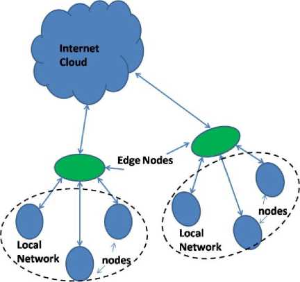
Fig. 7. Schematic of the database replication in network

• III.    Analysis of Algorithm and Mathematcial Framewok

As the replicated data is either available locally or it is available globally i.e., at the internet. Therefore, when request are generated, some of the generated request will be full-filled locally and leftover request will be fetched from internet (master node). In this section simulation framework is developed to estimate the average response time of all the transactions. In nutshell there are four processes in database replication:

• •    Request generation at the local node

• •    Request serving at the local node

• •    Network propagation

• •    Servicing at the remote site in the global network

The important network parameters are:

Loss Probability: It refers to the volume of data that is lost through a network, or in other words, the fraction of the generated requests which are lost.

Network Load: In networking, load refers to the amount of data (traffic) being carried by the network.

Network Delay: It is an important design and performance characteristic of data network. The delay of a network specifies how long it takes for a request to travel across the network from one node or endpoint to another. Delay may differ slightly, depending on the location of the specific pair of communicating nodes.

In Fig. 7, the generic layout of the database replication network is presented. Here, the local network is shown with dotted lines, and nodes sitting inside of the local network are shown with circular structure. The green oval shape represents the edge nodes where the data is aggregated and transferred to the global network. The global network is shown as internet cloud. In Fig. 8, the same network is again presented, here it is shown that the generated data can be served locally or can be transferred to the global network (red line).

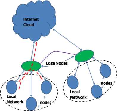
Fig. 8. Schematic of the database replication in network

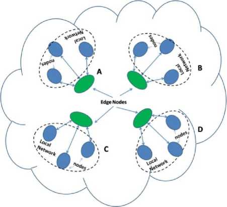
Fig. 9. Schematic of the database replication in network

In Fig. 9, a generalized topology of network is presented. As a network perspective, there is no distinction in local and global network and same queuing structure is applicable. Considering the Fig. 6, a request generated in cluster ‘A’ will treat cluster ‘A’ as LAN

(Local Area Network) and Clusters ‘B’, ‘C’ and ‘D’ will be a part of global network. Similarly, a request generated in cluster ‘D’ will treat cluster ‘D’ as local network while ‘A’, ‘B’ and ‘C’ will be treated as global network.

• A. Mathematical Description

Let in the local network r request are generated with probability p (it is assumed that each request are generated with equal probability), out of which l requests are served locally with probability p , then ( r — l ) requests will be transmitted to the outer world (global network). Hence, the request arrival rate X can be expressed as

X = rpr (1)

Then the mean value of the request served locally is

XL = Xp(2)

And the request served globally are

XG = X (1—p)

X = XL+xG(4)

X = rprp + r(1 - p) pr(5)

The throughput can be calculated as

T = (--gl tl + J_tg

Where, ‘g’ is fraction of packets served globally. The total delay can be evaluated as

D = D L + D G av      av

Thus it is evident from above discussion that the generated request first will be served locally and then globally. However the simultaneous request send to both local and global server will reduce the latency. Therefore in simulation two sets of parameters throughput and average delay are considered. As at the servers due to the pending requests queue may generate and this queue may in shard manner or it can be a dedicate queue as in output systems. If requested data is available at more than one server than the requests will be shared among them, thus this load balancing scheme not only reduce the average delay but also increases the throughput. Therefore simulation results are developed for shared, output queued systems with and without load balancing scheme. Finally, using these results network delay is estimated in section V.

• IV. Simulation Results

The simulation is done in MATLAB. The simulation pattern is based on random number generation and well known as Monte Carlo simulation. In the simulation random traffic model is considered. In the simulation we assumed the following

• 1.    Request can be generated at any of the input with probability p_r .

• 2.    With probability   p . the generated request served

• 3.    Each request is equally likely to go to any of the server

locally.

(locally or globally) with probability , where N is

N the number of server available.

The probability that K requests arrive at the particular server is given by

K   K        N - ^K

K ( N ) ( N)

In the simulation synchronous network is considered hence time is divided into slots. Therefore following assumptions are made

• 1.    The requests can be generated at the slot boundary only.

• 2.    Updates can be made at the slot boundary only.

• 3.    Once replication is started, then further updation is not allowed till replication complete.

• A.    Output Buffering

In Fig. 10-13, the results in terms of packet loss probability and average delay for output buffering is presented [10].

In Fig. 10, packet loss probability vs. load on the system is presented while assuming 4x4 node i.e., 4 input and 4 output and buffering of 4, 8 and 16 packets. It is clear from the figure as the load increases the packet loss probability increases. It can also be visualized form the figure that as the buffering capacity increases the packet loss probability decreases. At the load of 0.8, with buffering capacity of 16, 8 and 4 packets, the packet loss probability is — 3 x 10 5 ,-2 x 10 ³ and — 1.5 x 10 ² respectively.

Thus by increasing the buffer space by four fold i.e., from 4 to 16, the packet loss probability is improved by a factor of 2000. Therefore it can be summarized that the buffering capacity has deep impact on the over-all packet loss probability.

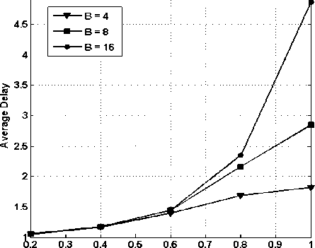
In Fig. 11, average delay vs. load on the system is presented while assuming 4x4 node i.e., 4 input and 4 output and buffering of 4, 8 and 16 packets. It is clear from the figure as the load increases the average delay increases. It can also be visualized form the figure that as the buffering capacity increases the average delay also increases. The average delay remains nearly same till load reaches 0.8 and in fact average delay is independent of buffering capacity. But as we cross 0.8 mark, the average delay shoots up. This is obvious as, at the higher load more number of packets will arrive means more contention, and thus in turn more buffering of packets.

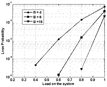
Fig. 10. Packet loss probability vs. load on the system with varying buffering capacity

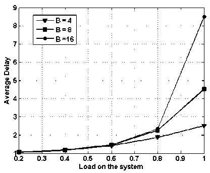
Fig. 11. Average delay vs. load on the system with varying buffering capacity

Load on the system

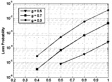
Fig. 12. packet loss probability vs. load on the system with fix buffering capacity of 4, with load balancing

In Fig. 12, packet loss probability vs. load on the system is presented while assuming 4x4 node i.e., 4 input and 4 output and buffering of 4 packets. However, load balancing scheme is applied. In the figure ‘ g ’ represents the fraction of traffic routed to global network. For ‘ g =0.5’ the packet loss probability, improves by a factor of 100 in comparison to ‘g=0.9’. Similarly, at the load of 0.6, the packet loss improves by 10 when g changes from 0.5 to 0.7 and similarly from 0.7 to 0.9.

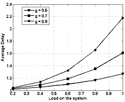
Fig. 13. Average delay vs. load on the system with fix buffering capacity of 4, with load balancing

In Fig. 13, average delay vs. load on the system is presented while assuming 4x4 node i.e., 4 input and 4 output and buffering of 4 packets. However, load balancing scheme is applied. In the figure ‘ g ’ represents the fraction of traffic routed to global network. Comparing with figure 11, the average delay has reduced considerably and this difference is more prominent at the higher loads. For ‘ g =0.5’ the average delay at the load one is reduced by nearly 7 slots. Similarly for ‘ g =0.9’, the average delay is recued by 6 slots.

• B.    Shared Buffering

In Fig. 14-17, results for shared buffering scheme are presented. In figure 14, packet loss probability vs. load on the system is presented while assuming 4x4 node i.e., 4 input and 4 output and buffering of 4, 8 and 16 packets. It is clear from the figure as the load increases the packet loss probability increases. It can also be visualized form the figure that as the buffering capacity increases the packet loss probability decreases. At the load of 0.8, with buffering capacity of 4, 8 and 16 packets, the packet loss probability is —4 x 10 2,— 9 x 10 3 and —1 x 10- 4 respectively.

Thus by increasing the buffer space by four fold i.e., from 4 to 16, the packet loss probability is improved by a factor of 400. In case of the output buffering at the load of 0.8, the packet loss rate is 3 x 10 5 , however in case of shared buffering the packet loss rate is —1 x 10- 4 . Therefore in case of output buffered system, packet loss better by a factor of three only. But in case of shared buffering the total buffer space is 16, but in case of output queued system is 64. Hence, the performance of the shared buffering is much superior to that of output queued system with much complex controlling algorithm.

In Fig. 15, average delay vs. load on the system is presented while assuming 4x4 node i.e., 4 input and 4 output and buffering of 4, 8 and 16 packets. It is clear from the figure as the load increases the average delay increases. It can also be visualized form the figure that as the buffering capacity increases the average delay also increases. The average delay remains nearly same till load reaches 0.6 and in fact average delay is independent of buffering capacity. The average delay is of 5 slots for B=16, which is much less that the output queued system (8.5 slots). Therefore, the average delay performance of the shared buffer is much better than that of output queued system.

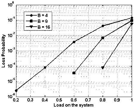
Fig. 14. Packet loss probability vs. load on the system with varying shared buffering capacity

Load on the system

Fig. 15. Average delay vs. load on the system with varying shared buffering capacity

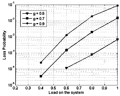
Fig. 16. Packet loss probability vs. load on the system with fix shared buffering capacity of 4, with load balancing

In Fig. 16, packet loss probability vs. load on the system is presented while assuming 4x4 node i.e., 4 input and 4 output and buffering of 4 packets in shared manner. However, load balancing scheme is applied. In the figure ‘ g ’ represents the fraction of traffic routed to global network. At the load of 0.6, the packet loss performance of the shared and output buffered system is nearly same (Fig. 12 and 16). Thus with much reduced buffering requirements shared buffering scheme, along with load balancing scheme provide very effective solution.

In Fig. 17, average delay vs. load on the system is presented while assuming 4x4 node i.e., 4 input and 4 output and shared buffering of 4 packets. However, load balancing scheme is applied. In the figure ‘ g ’ represents the fraction of traffic routed to global network. Comparing with figure 11 and 13 the average delay has reduced considerably and this difference is more prominent at the higher loads.

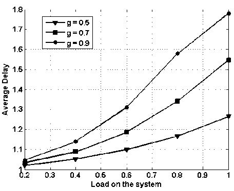
Fig. 17. Average delay vs. load on the system with fix shared buffering capacity of 4, with load balancing

• V.    Network Delay

When data request traverse through the network, the network delay may be significant, and it becomes an important delay parameter. If we incorporate the network delay ( D ), then the total delay will be formulated as

The total delay can be evaluated as

LG

D  Dav + Dav + DN I W

Here, D is the round trip delay.

Now as the more data centric applications are coming up, the whole computer network system is slowly transferring in fiber optic network.

Consider the fiber optic network and let the global node is 1000 Km away for the request generating node, then the latency in the network would be [11-14]

_ L Ln 1000 x1000 x1.5

D NIW = ” =    =      -  7718              AX

Therefore, the round trip delay would be 10 ms. Similarly, if a local node is only 100 m away from the request generating node then the round trip network delay would be 0.5 ps .

The latency this introduces is proportional to the size of the frame being transmitted and inversely proportional to the bit rate as follows:

F

BR

In the above equation, F is the frame size and B is the bit rate. For a frame of 64 bytes and data rate of 100 Mbps the delay is 0.5 ps . As average queuing delay is in terms of frame size, for example a delay of 8.5 slots (output queued system) will be    equal

to 0.5 X 8.5 = 4.25 ps and for shared buffering 0.5 x 5 = 2.5ps.

In case of global network, the main contribution in the delay is due to the propagation delay. Considering the case, when all the generated request are transferred to global network (refer figure 4.3) is

Again considering the case, when all the generated request are served at local network (refer figure 9) is

As there is no distinction for local and global buffering node, hence same buffering capacity should be considered.

In case of shared buffering,

Assuming that the data servers are employed separately in the network for data replication. As these data server will be fixed in numbers and they will have large buffering capacity. Considering the case of buffering of 100 requests, here the throughput will be very high and delay will also be larger. Assuming a delay of 50 slots, then the total delay would be

D = 0.5 ps x 50 + 20ms = 20.025ms.

• VI.    conclusion

In this paper, performance evaluation of a data base replication algorithm is presented in a fiber optic network. Simulation results are presented to obtain the mean waiting time and packet loss rate for shared and output buffered schemes. It is found form the results of the paper, that storage capacity has deep impact on the packet loss rate and average delay. If the load is below 80% then, nearly 100% throughput (1-packet loss rate) is possible with very small average delay (in slots), even at the higher load the throughput is very acceptable. The load balancing scheme further improves the results by bringing down both packet loss rate and average delay. Finally, the network delay analysis is presented for the complete estimation of the delay..