Let us consider a population divided into a finite number of classes with respect to some attribute, such as age, status, or geographical location. The state of the population at any time t can be described by the vector x(t) = (x 1 (t),... ,xn(t)). wlrere xi(t),i = 1,... ,n, gives the number of individuals with attribute i at time t. If we observe this population in discrete time then, in the linear case, its evolution can be modelled by x (k + 1) = A x (k), k > 0, x (0) = x, where x is the initial state of the population and the matrix A, often called the projection matrix, [1, Chapter 1], describes the transfers between the classes and changes in them between subsequent observations. It is commonly assumed in population theory that if a model is correctly formulated, then positive initial conditions should give a positive (or at least nonnegative) population at any later time. It is well-known, see e.g. [2, Section 6.1], that this is equivalent to all entries of A being nonnegative. However, it sometimes happens that reasonable assumptions on the population lead to projection matrices with entries of varying sign and this results in at least some trajectories eventually becoming negative. Nevertheless, it can happen that some initial conditions still give nonnegative trajectories. If we interpret an eventually negative trajectory as describing a collapse of the population (the population evolves soundly for some time but then it reaches a stage after which any further evolution within the framework of the model becomes impossible), then the initial conditions generating positive trajectories give rise to unbroken evolution of the population. The set of initial conditions (possibly empty) generating nonnegative trajectories will be called the viability set - of course any point on a nonnegative trajectory belongs to the viability set. Since it is determined by the entries of A, that typically reflect the environmental constraints, the viability set describes the constraints imposed by the environment on the structure of the initial population that ensure the survival of the population.

By linearity, if x and y generate positive trajectories. then so does a x + в У for any a, в >  0. Hence the viability set is a convex cone that we shall call the viability cone. Due to this, tools from convex analysis can be successfully employed to determine the viability cone for any A . In this paper we demonstrate this link between convex analysis, the Perron-Frobenius theory and population theory using the Natchez civilisation as an example.

We note that several Perron-Frobenius like theories have been developed for matrices with some negative entries, see e.g. [3] or [4] and references therein. Our model, however, does not satisfy the assumption of the former and thus we use the ideas of [4].

1.    The Model

Almost every society has more or less explicit class, or cast, system. In most societies the membership in a particular class is largely hereditary, through endogamy; that is, marrying within one’s own class. This has been the cause of many hereditary diseases, especially among aristocracy, where the available pool of potential spouses always has been limited. A relatively recent example is haemophilia suffered by many descendants of Queen Victoria. Despite this, the desire to provide for own children is so prevalent that few societies have decided to limit endogamy by practicing an open class system to prevent stagnation of the structure. An interesting example is offered by the civilization of Natchez.

Natchez were Native Americans who lived in the lower Mississippi in North America. Possibly the earliest European account of the Natchez is due to Hernando de Soto, whose expedition encountered a powerful chiefdom on the eastern bank of the Mississippi River in 1542 but was attacked by them and chased away. Most information about the Natchez civilisation has come from French colonists and missionaries who established contacts with them in the 17th century. The civilisation ceased to exist after the so-called Natchez revolt in 1729-1731, that followed three earlier wars with French; then Natchez were finally defeated and then dispersed or were enslaved.

French missionaries, explorers and colonial administrators recorded basic features of the Natchez’s social life. Their accounts were used by J. R. Swanton to write the first modern reconstruction of the Natchez society in 1911, see [5]. It turned out that Natchez had created a striking example of a stratified social system of open classes based on exogamous marriages so that the power was passed between people born to different social classes. The society was divided into two main classes - Nobility and Commoners (in early literature also called Stinkards). The Nobility was further divided into subclasses (casts): Suns, Nobles and Honoured. A member of Nobility only could marry a Commoner (but Commoners could marry within its own class). The inheritance of the class membership was matrilineal, with the exception that the children of Sun fathers were Noble, and the children of Noble fathers were Honoured. This description has created a lot of controversy due to the so-called Natchez paradox - as observed in [6], in this model the number of Nobles and Honoured would burgeon and the Commoner class would be depleted in successive generations until in the society there would be insufficient number of Commoners to provide spouses for the Nobility. We shall provide a quantitative illustration of this paradox in the next section. Since the Natchez civilization existed for several hundred years, according to [6], the Swanton model is biologically impossible. There were several attempts to explain this paradox, ranging from questioning the class inheritance rules to proposing different reproduction rates in each class, see [7, 8]. A first mathematical account of the latter approach can be found in [2, pp. 106-108, 174-178] and in this paper we shall propose a more general look at the problem along the lines sketched in op.cit.

2.    The Natchez Paradox

Following [2, pp. 174-178], we simplify the analysis by merging the Nobles and the Honoured into one class - say the Nobles. First, we summarize the rules for status inheritance in the table below.

Table 1

Possible marriages in the Natchez population and the status of their offspring

Mother \ Father	Sun	Noble	Commoner
Sun			Sun
Noble			Noble
Commoner	Noble	Commoner	Commoner

The following assumptions were commonly adopted in the literature.

• 1.    There is the same number of males and females in each class in each generation and we only track males.

• 2.    Each person marries only once and the spouse is from the same generation.

• 3.    Each pair has exactly one son and one daughter.

Let the population (of males) in the kth generation be described by x (k) = (x i( k) ,x2( k) , x з( k))

with the classes numbered as follows: 1 - Sun, 2 - Noble, 3 - Commoner.

Since a Sun son only can be born to a Sun mother and there is no other way to become a Sun, using the fact that the number of female Suns equals the number of male Suns we can write x 1( k + 1) = x 1( k).

A Noble son only can be born to Sun father or to Noble mother hence, using the parity of males and females in the Noble class, we get x 2( k + 1) = x i( k) + x 2( k).

Finally, the number of male offspring in the Commoner class is equal to the number of Commoner males who are not married to the females from the Nobility plus the number of sons of Commoner mothers and Noble fathers (remember that the son of a Commoner father and a Noble mother is a Noble but then the son of a Commoner mother and a Noble father is a Commoner). Hence xз(k + 1) = -xi(k) - x2(k) + x2(k) + x3(k) = -xi(k) + xз(k).

Writing the model in matrix form, we have x (k + 1) = Ax (k) = (I + B) x (k),     x (0) = x,

where

1 0 00 0 0

A=     1 1 0   , B=     1 0 0

-10 1

I is the identity matrix and x is the initial structure of the population.

We immediately see that this is not a correct population model in the conventional sense since the transition matrix A does not have positive entries and thus not all solutions ( x ( k )) _k> 0 of (1) with nonnegative x are nonnegative, see e.g. [2, Section 6.1]. In this case we can give a more detailed description. We see that B² = 0, he nee A ^k = I + k B; that is,

A ^k

k

-k

If x 1(0) = 0 , the structure of the population does not change since x ( k ) = (0 ,x 2(0) ,x 3(0)) .

If, however, originally we have some members of the Sun class, then the size of the Commoner class becomes negative in finite time. Indeed x ₃( k ) = —kx 1(0) + x 3(0) and thus x 1(0) >  0 vie Ids x ₃( k ) <  0 for k > x 3(0) /x 1(0). As discussed in Introduction, this can be interpreted as the dropping of the number of Commoners below the level allowing for all Nobles and Suns to marry before time k . This occurs for any initial condition with x 1 >  0, hence the civilisation in the described form cannot survive as Suns and Nobles have to marry Commoners. Since, however, according to the historical records, the Natchez civilisation with its social structure survived for several hundred years, the model in the presented form cannot be correct. As we noted in Introduction, several explanations have been presented to explain the paradox. We shall consider the suggestion of [7] that there were different birth rates in different casts.

3.    The Luenberger Solution

To our knowledge, the first attempt to mathematically analyse the Natchez population was done in [2]. The author followed the assumption discussed in [7] and asked the cpiestion whether it was possible find birth rates for each combination of parents in the Natchez community that would result in its positive stable class distribution? Consider the the intermarriage/fecundity scheme presented in Table 2, where ai >  0 , i = 1 ,..., 5 , is the average number of male offspring from such a marriage.

Modelling as before again leads to where this time

x ( k + 1) = A x ( k ) ,

	a 1	0	0
A=	a 2	a 3	0
	к -a 5	a 4 — a 5	a 5

Table 2

Intermarriage scheme in a simplified Natchez-like community with differential birth rates

Mother \ Father	Sun	Noble	Commoner
Sun			Sun а 1
Noble			Noble а 3
Commoner	Noble а2	Commoner а4	Commoner а5

Luenberger’s idea was to try to find out under what conditions there exists a positive eigenvector e о f A belonging to the large st positive eigenvalue A _max. This would show that in the long run the structure of the population stabilizes with each class remaining strictly positive,

x ( k ) = A ^k x ~ A^k _max ( e* , x ) e , for large k, (3)

provided ( e *, x ) = 0, where by ( ■, ■ ) we understand the standard dot product in R ⁿ and e * is the (normalized) left eigenvector of A.

The weakness of this solution is that the existence of a positive eigenvector belonging to the dominant eigenvalue does not ensure that the population will reach this state through strictly positive iterations. This problem is addressed in the next section.

Let us return to Luenberger’s solution. Since the matrix A is triangular, its eigenvalues are given by а 1, а3 and а5. If а5 is the dominant eigenvalue, then the long term structure is given by e = (0, 0,1); that is, the population will only consists of Commoners. While it is certainly possible, we are interested in the survival of the community with the original structure, which clearly is not possible in this case. A similar outcome is obtained if we assume that а3 is the dominant eigenvalue. Then the stable population structure is e = (o, 1, 0)3-05) , Provided а4 > а5. Finally, if а 1 is the dominant eigenvalue, stable population structure is given by then the

e

=0 •

α 2

α ₁ - α ₃

α ₁ - α ₅

α ₄ - α ₅

-а 5 + а 2------

α 1 - α 3

and it is positive if and only if а2(а4 — а5) > аз(а 1 — а3).

То complete our considerations, we must show that in the stable structure we have sufficiently many Commoners for the Suns and Nobles to marry; that is, that the coordinates of e satisfy x3 - x 1 + x2. (6)

Substituting here the formulae for x2 and x 3 , which were derived earlier, we obtain

1               а4 — а5

00-05 fo“5 + 0200-03) - 1 +(00-03)• that yields the inequality [2, Equations (5-81)], а4 — а5   а5(а1 — а3) а1 — а3

7 о---1 - 0.(o)

а1 — а5   а2(а1 — а5)

This inequality will be satisfied if a4 is sufficiently large. For instance, the choice a 1 = 1 . 1 , a 2 = 1 . 0 , a 3 = 1 . 0 , a 4 = 1 . 3 , a 5 = 0 . 9 works, giving the stable population distribution as e = (1 , 10 , 15 . 5) . In general, if the fecundity in marriages of Commoner mothers and Noble fathers should be sufficiently large, then we have sufficiently many Commoners in the stable population distribution.

4.    Full Solution

As we have mentioned earlier, the provided analysis is not complete as it only shows that there is a structure of the society which can persist in a stable way. However, we do not know whether any positive initial population satisfying (6) will give rise to a positive population satisfying (6) in each generation, that will eventually stabilize at the structure determined by the eigenvector found above.

Fortunately, the problem allows for a more detailed solution which confirms the results obtained by the analysis of the dominant eigenvalue and the corresponding eigenvector. To avoid dealing with several subcases, here we assume that a 1 >  max {a 3 , a 5 } and a 3 = a 5.

For the solution with x 1 > 0 we have xi(k) = akx 1 > 0,    x2(k) = akx2 + a2x 1 —---— > 0.

• ^{1                       3}           α ₁ - α ₃

  Further

  
  

  ^α

  x з( k ) = a ₅ x 3 +-- ^α 3 ^-

  ₊ ok-a

  α ₁ - α ₅

  
  

  ^k α ₅

  α ₅

  
  

  ( a ₄ - a ₅) x ₂

  
  

  - x _i

  α 1

  
  

  a 2( a 4 - a 5)

  - α 5 x 1 .

  α 1 - α 3

  
  

  α 2

  - α ₃

  
  

  )

  
  

  +

  
  
  
  

Hence x3(k) is nonnegative provided (5) is satisfied and x i   a i — a з

x 2       a 2

In other words, for the solution to remain positive, the ratio of the initial population of Suns and Nobles should be smaller than the ratio of these populations in the stable population distribution vector. Furthermore, for the population structure to persist, there must be enough Commoners for the Nobility to marry, so that we need ( x _i( k ) , x 2( k ) , x ₃( k )) to satisfy (6) for any k. In principle, it is possible to prove it from (9) but it requires lengthy calculation. There is, however, a smarter and systematic way to do this that uses the concept of cross-positive matrices [4, 9].

Let us recall the definition of a cone used in the results below. We say that C C R ⁿ is a cone if C is nonempty, closed and satisfies C + C C C. aC C C for all a >  0 , C — C = R ⁿ and C П ( —C ) = { 0 } . Our problem can be re-formulated as follows: find ( a 1 ,..., a 5) G R+ such that the cone in R+ , determined by (10) and (6); that is

C =

{( x i ,x 2 ,x 3); x i >  0 ,

-------x _i + x 2 >  0 , x 3 > x _i + x 2 α 1 - α 3

,

remains invariant under A, A C C C, where A is defined bу (2). Cone C , see Figure, is the viability cone for the Natchez population, as defined in Introduction.

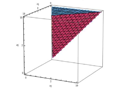
The viability cone C

We need the concept of a polar set.

Definition 1. The polar set S* of a non-empty set S гn R ⁿ is defined to be

S* = {z E R ⁿ ; ( z, y) >  0 for all y E S}.

It follows that if C is a cone in R ⁿ, then so is C* [10, Chapter I §4]. Furthermore, C** = C [see [10, Corollary to Theorem 3 of Chapter I] or [4, Lemma 2]). Then we have

Proposition 1. [4, Remark 1] Let C be a cone in R ⁿ a nd A be an n x n matrix. Then A C C C if ami only if ( z , A y ) >  0 for all y E C, z E C*.

We recall some necessary terminology. Let a 1 ,..., a r and b 1 ,..., b _s be some vectors In R ⁿ. We say that a, cone C C R ⁿ Is polyhedral if

C = { x ;( a j, x ) >  0 , j = 1 , ...,r}                       (12)

and that it is finitely generated if s

C = { x ; x = ^pj b j, pj >  0 , j = 1 , ..., s} =: cone ( { b 1 ,..., b _r} ) .        (13)

j =1

We observe that if C is polyhedral then, from the definition of the cone, Span{ a j}j =1 ,...,_r = R ⁿ . Indeed, otherwise there would be 0 = x ± Span{ a j-}j =1 ,...,_r . Then, by definition, x E C but. since ( a j, x ) = 0 , x E C П ( —C ) and 1 ieiice x = 0.

The main result of the paper is

Theorem 1. Let ai ,i = 1,..., 5, be positive, q := max {a 3, a 5}/a 1 < 1 and a i( a i — a 3 + a 2)

^α 4 ≥

α 2

Then the. coin?. C defined by (И) i. s invariant under A and. for x E C with x 1 >  0.

A k x              a 2       1                a 4 — a 5           k.

= x 1  ¹ ,          ,           I ^—a 5 + ^a 2          I I + O ⁽ q ) . (Io)

α ⁵₁            α 1 - α 3 α 1 - α 5             α 1 - α 3

Proof. It is easy to see that

C = {x; (ai, x) > 0, (a2, x) > 0, (a3, x) > 0}, where

a 1 = (1 , 0 , 0) ,

^a 2 ⁼

α 2

a 1 — a 3

1 , 0^ ,

a 3 = ^{( — 1} , ^{— 1} , 1) •

From the Minkowski-Weyl theorem, [11, Theorem 19.1], a cone is polyhedral if and only if it is finitely generated with the vectors { b i} =1 ,...,s of (13) being the extreme rays (directions), op.cit. In our case, since Span{ a j}j =1 ,2, 3 = R³ and { a j}j =1 ,2, 3 are linearly independent, it is easy to see that a bi-orthogonal system of vectors { b i} =1 ,2, 3; that is, satisfying ( a j, b i ) = 5ij,i,j = 1 , 2 , 3 , (the Kronecker delta) can be taken as generating C. Indeed, let

3 x' = 52 (ai, x)bi- i=1

Then

( a j, x — x ) = ( a j, x ) — 52( a i, x )( a j, b i ) = 0 , j = 1 , 2 , 3 , i =1

and, since Span{aj}j=1,2,3 = R3, x = x'. Thus, if x G C, it can be expressed as a nonnegative linear combination of {bi}i=1,2,3• Conversely, if x = 52 ^ibi’ ^i > 0,i = 1, 2, 3, i=1

then (aj, x) = pj > 0 and hence x G C. Since we are in R3, such vectors are the normalized cross products b 3 = a 1 x a 2 = (0, 0, 1), b 2 = a 3 x a 1 = (0, 1, 1), b 1 = a 2 x a 3 = (1, ———, 1 +--a2— ) , a1 — a3     a1 — a3

thus

C = cone f Я1 ,-a2—, 1 +   'V (0, 1, 1), (0, 0, 1)}У a1 — a3     a1 — a3

To End C*. we use the Farkas lemma. [11. Corollary 22.3.1] that states that if C = cone ( { a 1 , • • •, a r} ) , then

C* = {x; (aj, x) > 0, j = 1 ’•••’r} and

{ x ; ( a j, x ) >  0 , j = 1 , • • •, r}* = cone ( { a 1 ,• • •, a r} ) •

Thus,

C* = { y ; ( b 1 , y ) >  0 , ( b 2 , y ) >  0 , ( b 3 , y ) >  0 } = { x ; ( a 1 , x ) >  0 , ( a 2 , x ) >  0 , ( a 3 , x ) >  0 }* = cone ( { a 1 , a 2 , a 3 } ) •

We need to prove ( y , A x ) >  0 for all y E C*, x E C. However, it is clear that it suffices to check

( a i, A b j ) >  0 , i,j — 1 , 2 , 3 .

This gives 9 inequalities to check. First, we have

A b 1

^a i , a 2 +

a 2 a з a 1 — a 3

a 2 a 4

a ₁ — a ₃

,

A b 2 = (0 , a з , a 4) ,

A b 3 — (0 , 0 ,a 5) .

Hence

( a 1 , A b 1) = a 1 ,   ( a 1 , A b 2) = 0 ,   ( a 1 , A b 3) = 0 ,

(a2, Ab1) = 0,   (a2, Ab2) = a3,   (a2, Ab2) = 0, a 1( — a 1 + a 3 — a 2) + a 2 a 4

⁽ a 3 , A b 1) = ----------------------------- ,   ⁽ a 3 , A b 2) = ^a 4 ^{— a} 3 ,   ⁽ a 2 , A b 2) = ^a 5

a 1 — a 3

resulting in a4 > a3,

a i( a 1 — a 3 + a 2)

a 4 >-------------- a2

However, since a 1 > a 3. (17) yields

_ a 1( a 1 — a 3 + a 2)    a s( a 3 — a 3 + a 2)

a 4 > -------------- > --------------— a 3

a 2                   a 2

so that (16) is superfluous.

Then (15) follows from (4) and (3) as e * — (1 , 0 , 0) is the normalized left eigenvector belonging to a 1.

□

Remark 1. We observe that (14) seems not to be related to (5) and (8). Though the latter can be inferred from the former indirectly, since C is closed and e can be obtained as the limit of iterations of (A/a5)kx as k ^ to with x E C, we also provide a direct proof. Since a 1 > a5. from (17) we have a2a4 > a5(a1 — a3 + a2)

so that (17) yields (5). Further, a1 — a3 + a2 —

( a 1 — a 3)  1 +

a -2

a ₁ — a ₃

)

hence, using twice (17),

a

0 < 1 +---2— < a1 — a3

a 2 a 4

a ₁( a ₁ — a ₃)

( a 1 — a 5) a 2 a 4 a ₁( a ₁ — a ₅)( a ₁ — a ₃)

1                      a 2 a 4^ /     .V.    _ 4   a 2 a 4   a 5 ( a 1 - a 5)( a 1 - a 3)               a 1

< a 2 a 4 - a 5( a 1 - a 3 + a 2) ( a 1 - a 5)( a 1 - a 3)

Thus (8); that is,

α ₁ - α ₅

α ₄ - α ₅

-a 5 + a 2------

α 1 - α 3

α

> 1 +---²— >  0

α ₁ - α ₃

also is satisfied.

Acknowledgement. The research was supported by the National Research Foundation of South Africa under Grant NN. 0031 7.