Potentials allowing integration of the perturbed two-body problem in regular coordinates

POTENTIALS ALLOWING INTEGRATION OF THE PERTURBED TWO-BODY PROBLEM IN REGULAR COORDINATES

Syktyvkar

The integrable cases of motion equations have great practical value. Their significance is determined by the fact that with the help of their solutions one can analyze the motion. In a number of cases integrable problems are used to construct intermediate orbits [1,2]. One of non-trivial examples of integrated systems is the particle motion in a Newtonian field with additional constant acceleration vector. This had been investigated earlier by a number of authors [3–5] and applied to analysis of space flights with constant jet acceleration. In 1970, this problem was studied using regular coordinates obtained from the KS-matrix [6]. In contrast to [6], in [7] integration of the same problem was performed in regular coordinates obtained with the use of L -transformations.

In the present work we consider a problem of constructing potentials allowing integration of the equations of motion. The idea of our approach consists in the following. First, a new dynamic system is constructed, having more degrees of freedom than the original one. To do this, an L -transformation is applied. The theory of L -matrices and their applications is given in [8, 9]. Using new coordinates, a general potential is selected, allowing separation of variables in the Hamilton - Jacobi equation. After this, an inverse transform to original coordinates is performed, using explicit formulas. As a basis for selecting general potential with the required integrability property, a well known Stackel theorem is used [10]. This theorem gives necessary and sufficient conditions for separation of variables for orthogonal Hamilton systems, i.e. systems whose Hamiltonian contains only squares of generalized momentums.

Note that separation of variables depends on a choice of a coordinate system. We consider here three kinds of coordinate systems: regular, bipolar and spherical. The last two systems are introduced in regular coordinates. Canonical equations in regular coordinates are constructed using arbitrary L-transformations from the initial canonical motion equations of the perturbed two-body problem. The new equations have also orthogonal form and are invariant with respect to L-similarity transforms. In the nonperturbed case these equations do not have singularity at the attracting center. Due to invariance with respect to some perturbing potentials allowing integrability, one can introduce two additional angular parameters.

As a result of this approach the general solution of original system is represented in parametric form, where fictitious time plays the role of parameter, while the physical time depends on this fictitious time and initial data. This sort of integrability is sometimes called ’Sundman integrability’ [11].

As an example of integrable case of the perturbed two-body problem the special kind of potential is given. In this example the explicit solution of the problem in terms of elliptic functions is expressed, and the criterion of bounded motion is formulated.

Notation . Everywhere below vectors are regarded as column vectors, and are given in bold letters. The sign ^T placed over the vector or matrix symbol denotes transposition. A quantity evaluated at the initial moment of physical or fictitious time is denoted by zero superscript: f (0) = f 0 .

1. The separation of variables

Let us consider the Hamiltonian function of the perturbed two-body problem

H = H(x, y ) = 2 | y | ² - ^ + V,

P = Y ( m + m o ) , r = I x I,           (1)

where x = ( x 1 , x 2 ,x 3 ) T is the position vector of the point of mass m with respect to the point of mass m 0 ; У = ( У 1 ,y 2 ,У з ) T is the generalized impulses ( y i = x i , i = 1 , 2 , 3 ); y is the gravitational constant; V = V(x) is the perturbed potential.

For construction of the equations of motion in regular coordinates we will need the L -transformation z = L ( q ) q generated by the L -matrix of the fourth order that has the following properties:

l ( q ) L T ( q ) = L T ( q ) l ( q ) = I q I ² e v q 6 R 4 , (2)

( l ( q ) p ) i = ( l ( p ) q ) i , i = 1 ,---,p,      (3)

( L ( q ) p ) i = - ( L ( p ) q ) i , i = p + 1 ,•••, 4    (4)

∀ q , p ∈ R ⁴ .

Here E is the unitary matrix. The conditions (2) – (4) simultaneously hold only for p = 1 or p = 3 . The quantity p is the rank of L -transformation. The following theorem can be proved [8, 9].

Theorem 1. An arbitrary L -matrix generating L -trans-formation of rank three, has the form

L ( q ) =

q ^T K 1 K 4 q ^T K 2 K 4 q ^T K 3 K 4 q ^T K 4

where orthogonal skew-symmetric matrices

K 1 , K 2 , K 3 , K 4 are equal to either

Ki = a i iU + a 2 i V + a 3 i W, i =1,2, 3, K4 = a 1X + a 2 Y + a 3 Z, or

K i = a 1 i ^{X +} a 2 i Y ⁺ a 3 i ^Z,  i = ¹ , ² , ³ ,

K 4 = a 1 U + a 2 V + a 3 W.

The triplet of vectors e i = ( a 1 i ,a 2 i ,a ₃ i ) ^T , i = 1 , 2 , 3 , forms an orthonormal basis in R ³ , and e = ( a 1 , a ₂ , a ₃ ) ^T is an arbitrary unitary vector.

Conversely, the arbitrary four skew-symmetric matrices in the form (6) or (7) define the L -matrix by the formula (5) .

In the formulae (6) and (7) there are the so-called basic skew-symmetric orthogonal matrices

	0 - 1 0			0
U =	1 0	0 0	0 0 -	0 1
	0	0	1	0
	0	0	0 -	1
W =	0 0	0 1	1 0	0 0
	1	0	0	0
	0	- 1	0	0
Y = 1	1 0	0 0	0 0	0 1
	0	0	- 1	0

/0 0 -1 0\ 0    0   0 1

=   1   0   0 0

0 -1   00

0 0 -10

0 0   0

= 10  00 L

01  00

0 0 0 - 1

0 0 1 0

= 0 - 10 0 •

\1 00 0/

The matrices K _i are called generators of the L -matrix. If K ₁ , K ₂ , K ₃ , K ₄ are calculated by the formulae (6) then L ( q ) is called the L -matrix of the first type , otherwise the L -matrix of the second type .

We transfer from variables t, xi , yi to the new variables τ , qj , pj by the formulae dt = r dT,

( x = Л( q ) q ,

I y = ^qp^л( q ⁾ p , q , p ⁶ R ^{4        (8)}

where the matrix Л( q ) is found from (5) by rejection of the fourth line:

q ^T K 1 K 4

Л(q) =   qT K2 K4   • qT K3 K4

Consider the equations of motion in new variables q i , p i

-

dq j ∂ K dp j dτ ∂p j dτ

dK, j = 0, 1,2, 3, 4 (9) ∂qj with the Hamiltonian

K = ¹ 1 p 1 ² + p 0 1 q 1 ² + I q 1 ² V c ( q ) , о

V c ⁽ q ) = V ( ^{x (} q )) •

In this system the first equation with j = 0 corresponds to transformation of time: dq 0 = | q | ² dT . The variable p 0 is conjugate to q 0 and has a constant value.

If

x (0) = x ⁰ , y (0) = y ⁰           (11)

are initial conditions for the variables of the system with the Hamiltonian (1), then, as it is proved in [12, 13], with the initial values defined by formulae

J qo(O) = 0,             x0 = Л(q0)q0, t p0(0) = —H(x0,y0), p0 = 2ЛT(q0)y0, the solution of (9) becomes, under the transformation (8), a solution of the system with the Hamiltonian (1) satisfying the initial conditions (11). The function qTK4p preserves a constant value along solutions of (9), and with the initial conditions from (12), this value is zero [13]. Hence, the equality qTK4p = 0 is the first integral of this system. The variable q0 coincides with physical time t.

Note that the systems with Hamiltonian (1) and (10) have different orders. The choice of initial values by the formulae (12) means that there is a special construction of the system (9) for each trajectory of the system with Hamiltonian (1).

Let’s pick up the form of potential V , admitting division of variables. For this purpose we shall take advantage of the theorem proved by Stackel [10].

Theorem 2. The system with Hamiltonian

n

H =

£ C i ( q 1 ,..., i =1

Q u )( 2 P 2 + V i ( q i )) ,

admits separation of variables in the Hamilton - Jacobi equation if and only if there is a nonspecial matrix Ф of order n which elements φ si depend only on q i , such as

Ф c = (1 , 0 ,..., 0) ^T ,             (13)

where c = ( c 1 , c 2 ,..., c _n ) ^T .

In this case the integrals of motion will be t - β1

n ^{q i}

= X i=1

q _i ⁰

Ф1 i (qi) dqi P fi ( qi ) , n   qi

-в‘=X/ qi0

Ф si ( q i ) dq i p f i ⁽ q i ) ,

s = 2 ,..., n,

Pi = Pfi (qi), i =1 ,...,n, where fi(qi) = 2(а 1 ф 1 i(qi)+.. . + anф^(qi)-Vi(qi)); ai, ei (i = 1,... ,n) is constant. As q0 a simple root of the function fi(qi) is taken.

Consider again the separation of variables in regular coordinates qi. The Hamiltonian looks like (10). In this case we have c 1 = C 2 = C 3 = C 4 = 4 ,

| q | ² ( p 0 + V c ( q )) = ₄£ V s ( q s ) .

s =1

The solution of system (13) will be, for example, the matrix

- 1

- 1

- 1

The potential is defined up to a constant. As p 0 is a constant, we obtain

V c ^{( q )} = 4 | q | 2 ⁽ V 1 ^{( q} 1 ) ⁺ V 2 ^{( q} 2 ^{) +}

^{+ V} 3 ^{( q} 3 ) ^{+ V} 1 ( ^q 4 )) . ⁽¹⁵⁾

Let’s find expression for the potential V c ( q ) in original coordinates x . We notice that variables x i and r are quadratic forms of the variables q 1 , q 2 , q 3 , q 4 . Using the L -similarity transformation it is possible to choose an L -matrix such as a linear combination B 1 x 1 + B ₂ x ₂ + B 3 x 3 that will be equal to the sum of squares of q i with some coefficients. Note that for any L -matrix we have r = | q | 2 . As V c ( q ) is to be of the form (15), the required potential in x -coordinates will be the function of the form

V ( x ) = r ( Ar + B 1 x 1 + B 2 x 2 + B 3 x 3 ) .    (16)

Let’s specify a choice of L -matrix with the required property. Introduce the notation

B = B 2 + B 2 + B 2 , b i = BB i , i = 1 , 2 , 3 .

Suppose that the L -matrix is of the first type. That is, K 1 , K 2 , K 3 are calculated by the formula (6); for simplicity we assume that K ₄ = —Y . Then

Ar + B ( b 1 x 1 + b 2 x 2 + b 3 x 3 ) =

= Ar - B q ^T [( b 1 a 11 + b 2 a 12 + b 3 a 13 ) U +

+ ( b 1 a 21 + b 2 a 22 + b 3 a 23 ) V +

+ ( b 1 a 31 + b 2 a 32 + b 3 a 33 ) w] Y q .

Choose the parameters a ij of L -matrix in such a way that the following equalities hold:

b 1 a 11 + b 2 a 12 + b 3 a 13 = 1 ,

< b 1 a 21 + b 2 a 22 + b 3 a 23 = 0 ,         (17)

b ₁ a ₃₁ + b ₂ a ₃₂ + b ₃ a ₃₃ = 0 .

Geometrically, the solution to this system means that the vector i1 = (a 11, a 12, a 13)T coincides with b = (b 1 ,b2, b3)T, and the vectors i2 = (a21 ,a22 ,a23)T, i3 = (a31, a32, a33)T are orthogonal to b. Moreover, it follows from the structure of the L-matrix that vectors i1 , i2, and i3 form a frame. It is evident that the system (17) has infinite number of solutions. We write its general solution. For the first vector we have i1 = (b 1 ,b 2 ,b 3)T.

For i2 and i3 we assume, in the case b 1 + b2 = 0, that i2 = —       (b2 cos a + bibз sin a, —b 1 cos a+

V b 1 + b 2^v

+ b 2 b з sin a, — ( b 1 + b 2 ) sin a) ,

We obtain

i ₃ = —        ( —b ₂ sin a + b ₁ b 3 cos a, b 1 sin a +

V b 1 + ь 2 V

+ b ₂ b 3 cos a, — ( b 1 + b 2 ) cos a) .

д Ф q 1 = 5- ∂p 1

д Ф q 2 =

∂p 2

д Ф q 3 =

∂p 3

дФ q 4 = 5-∂p4

д Ф

^{P 1} =

∂Q 1

V Q 7 cos Q 2 ,

VQ1 sin Q 2, x/Qs cos Q 4,

V Q a sin Q 4 ,

1 2 VQ 7

( P 1 cos Q 2 + P 2 sin Q 2 ) ,

If b 1 + b 2 = 0 , then b = (0 , 0 , b 3)^T , b 3 = ± 1 . Therefore, we can take the following vectors as the general solution of the system (17):

i 1 = (0 , 0 , b 3 ) ^T ,   i ₂ = I cos a, sin a, 01

i 3 = b 3 — sin a, cos a, 0    .

The quantity a G [0 , 2 n ] plays the role of an arbitrary parameter of the general solution.

After choosing the parameters a ij , the matrix A( q ) is determined uniquely. The solution of (17) gives

V^е ( q )= 1 ё 1 1 2 ( A* q ' ² —B q ^T uy q )=

= i q [ 2 (⁽ A ⁺ B ) ^q 1 ⁺⁽ A ⁺ B ) ^q 2 ⁺

⁺⁽ A—B ) q 2 ⁺⁽ A—B ) q 4 ) .

Hamiltonian in q -coordinates corresponding to this potential becomes

K 52 4 (2 p ^{2 + 4} p 0 q ^{2 + 4} D t q ²^) , i =1

where D1 = D2 = A + B, D3 = D4 = A — B. The canonical system of the equations falls into four subsystems di = 7Pi, dpi = — 2(P0+Di)qi, i = 1,2,3,4. (18) dT 4 dT

These systems are equivalent to four harmonious oscillators. Integrals of motion are obtained either from (14), or directly from solving (18). Thus, separation of variables for potential (16) is carried out.

For regular q -coordinates, we introduce a new coordinate system. To preserve the canonical form of equations of motion, we use the canonical transformation with generating function

Ф = p 1 VQ 1 cos Q 2 + P 2 V Q sin Q 2 +

P 2

P 3

P 4

д Ф ∂Q 2

д Ф ∂Q 3

д Ф ∂Q 4

V Q 7 ( —P 1 sin Q 2 + p 2 cos Q 2 ) ,

1 2 V0 3

( P 3 cos Q 4 + P 4 sin Q 4 ) ,

V Q 3 ( —p 3 sin Q 4 + p 4 cos Q 4 ) .

The coordinates Q ₁ , Q ₂ , Q ₃ , Q ₄ , obtained from (19), will be called bipolar. From the last four equations we find p 1 , p 2 , p 3 , p 4 :

p 1	= 2 Pn	/0 1 cos Q 2 —	P 2 √ Q 1	sin Q 2 ,
p 2	= 2 P 1	/Q 1 sin Q 2 + ■	P 2 √Q 1 P 4	cos Q 2 ,	(20)
	= 2 P 3	/ Q 3 cos Q 4 —		sin Q 4 ,
p 3			√ Q 3
p 4	= 2 P 3 VQ 3 sin Q 4 + •		P 4 √Q 3	cos Q 4 .

In the new variables the Hamiltonian K becomes

K = - (4 Q 1 P 1² + -2 + 4 Q 3 P 3² + -4 ) +

8 \           ^Q 1              ^Q 3/

+ p o(Q1 + Q 3) + (Q1 + Q 3) V, where function V is expressed in terms of Qi .

Similar to the above, consider separation of variables in bipolar coordinates. In the notations of theorem 2 we now have

C 1 = ^Q 1 , c 2 = -777-, c 3 = ^Q 3 , ^c 4 = 777.

4 Q ₁                   4 Q ₃

As a solution to (13) one can take the matrix

		1 Q 1	0 1	0 0 \
				00
Ф =		4 Q 1 21		1 Q	.       (21)
		- Q 1	0	Q 3 0
		0	0	— 4 Q 1 J

+ P 3 VQ 3 cos Q 4 + P 4 VQ 3 sin Q 4 .

For the potential V admitting separation of variables, we find

the form

V = о      ( ^Q 1 V 1 ^{( Q} 1 ) ⁺ ITTV 2 ^{( Q} 2 ^{) +}

Q 1 + Q 3 ^v            4 Q 1

+ Q з V з ( Q 3 ) + ^ V 4 ( Q 4 )) .

4 Q 3

In q -coordinates we obtain the form

P ²

K = Q 1 ~2^⁺ p 0 ⁺

+ Q 3

V c =

j qp ( ⁽ q ^{2 +} q 2 ) V 1 ⁽ q ^{2 +} q 2 ^{) +}

V 2 (arctan q i )

4( q ² + q 2 ) ⁺

^{+ ( q 2 + q 2 )} V з ^{( q 2 + q} 2 ) ⁺

V 4 (arctan q 3) \ 4( q 2 + q 2Т ' '

Passing to x -coordinates, we use the concrete L -trans-formation

( x 1 =   2 q 1 q 4 + 2 q 2 q 3 ,

< x 2 = - 2 q 1 q 3 + 2 q 2 q 4 ,            (22)

I x 3 = q 2 + q 2 - q 2 - q 4 ,

which follows from (5), (6) with K 1 = V , K ₂ = W , K 3 = U , K ₄ = —Y . Taking into account that for any L -matrix the equality r = q 2 + q 2 + q 2 + q 4 holds, we obtain

q ^{2 +} q 4 = |( r^{- x} 3 ) , q ^{2 +} q 2 = |( r ^{+ x} 3 ) .

The general solution of the first equation is

q 3 = V r 2 x ³ cos ^’ q 4 = r ₂ x ³ sin ^’ ^ G [0 , 2 n ] .

Then x 1 sin ^ — x2 cos ^        x 1 cos ^ + x2 sin ^

q ¹     v Vr - x 3    , q ²      v Vr - x 3

In a similar way we may introduce a parameter, using the second equation,

q 1 = V r ⁺ ₂ x ³ c°s ^ 1 ,  q 2 = ^/ r ⁺ ₂ ^{x 3} sin ■ф 1 ,

^ 1 G [0 , 2 n ] .

As is well known [12], with L -transformation for a point in R ³ at a distance r from the origin , there corresponds a point of some circle of radius ^√r in R ⁴ . The variables q i contain an arbitrary parameter ψ (or ψ 1 ), giving parametrization of the given circle. In the original coordinates x _i this parameter disappears. Note that

— = tan ^ 1 , — = tan ^. q 1                q 3

We therefore assume functions V ₂ , V ₄ to be constant. Then we arrive at a potential of the form

V ( x ) = 1 [ G 1 (( r + x 3 ) / 2) + G 2 (( r - x 3 ) / 2)] , (23)

where G ₁ , G ₂ are arbitrary smooth functions. The Hamiltonian in bipolar coordinates for this potential takes

G 1 ( Q 1 ) \

Q 1

P ²

"1" + P 0 +

+

1 P-2 ² --² +

4 Q 1 2

G 2 ( Q 3 ) \

Q 3

+ 1 P 2

⁺ 4 Q 3 2 .

In view of the solution (21) for f _i from the theorem 2 we have

f 1 ( q 1 )=2( a 1

Q 1

-

α 2

4 Q 2

α 3

Q 1

-

p 0 ^-

G 1 ( Q 1 )

Q 1

f 2 ( Q 2 ) = 2 a 2 ,

f з ⁽ Q 3 ) = ²( a r ^- 5742

Q 3   4 Q ₃

- p 0

-

G 2 ( Q 3 ) \

Q3     , f4 (Q4) = 2a4 .

Then integrals of motion are obtained by formulas (14).

Let’s consider one more case of separation of variables. Introduce the spherical coordinates in q -co-ordinates

q1 = q2 = q3 = q4 =

y Q 1 cos Q 2 cos Q 4 ,

V Q 7 sin Q 2 cos Q 4 ,

V Q 1 cos Q 3 sin Q 4 ,

V Q 1 sin Q 3 sin Q 4 .

We supplement the transformation (24) to obtain a canonical transformation of impulses

P 1 = 2 Vq1 cos Q 2 cos Q 4 P 1 -

-

sin Q 2

V Q 7 cos Q 4

P 2 ^-

cos Q 2 sin Q 4

Q 1

P 4 ,

P 2 = 2 VQ 1 sin Q 2 cos Q 4 P 1 +

+

cos Q 2

V Q 7 cos Q 4

P 2 ^-

sin Q ₂ sin Q ₄

Q 1

P 4 ,

P 3 = 2 VQ 1 cos Q 3 sin Q 4 P 1 -

sin Q 3

V Q 1 sin Q 4

P 3 +

cos Q ₃ cos Q ₄

Q 1

P 4 ,

P 4 ⁼ 2 VQ 1 sin Q 3 sin Q 4 P 1 +

cos Q 3

V Q 1 sin Q 4

P 3 +

sin Q 3 cos Q 4

Q 1

P 4 .

Then in new variables the Hamiltonian will be

K = ¹ (4 Q 1 P 1 ² + О X

P ₂²          P ₃ ²

Q 1 cos ² Q 4   Q ₁ sin ² Q ₄

P 4

⁺ Q 1/

+

⁺ p 0 ^Q 1 ^{+ Q} 1 V.

In the notations of Stackel theorem we have

c 1 ^Q 1 , c 2      .                ,

4 Q ₁ cos ² Q ₄

,              1             „        1

^:3 = 4 Q 1 sin ² Q 4 , c ⁴ = 4 Q 1 .

In this case the solution of (13) will be the matrix

Taking into consideration matrix (26), we then obtain

ф =

Q 1

-

-

cos^ Q 4

.

\

sin ² Q 4

4 Q 2

-

/

The potential V , admitting separation of variables, can be written as

V =     ( ^Q i V i^{( Q} i ) ⁺ 775----257” V 2^{( Q} 2⁾⁺

Q 1               4 Q 1 cos ² Q 4

⁺ 775 . 2_a V 3 ^{( Q} 3 ) ⁺ 775” V 4 ^{( Q} 4 )) •

4 Q 1 sin ² Q 4           4 Q 1

In view of relations

Q i cos ² Q 4 = q 2 + q 2

Q i sin ² Q 4 = q 2 + q 4

r + x 3 2

r-x 3

α 1     α 4

f ^{1 ( Q 1 )} = ²V Q i + 4 Q 1 ^- p ^{0 -}

G i ( Q i )

Q 1

f 2 ( Q 2 ) = 2( a 2 - 4 A ) , f 3 ( Q 3 ) = 2( a 3 - 4 B ) , f ^{4 ( Q 4 )} = ²( ^- coiQ^- s5 Q : ^-

- a 4 - 4 G 2 (cos 2 Q 4 ) •

The integrals of motion follow from (14).

Note that using an arbitrary L -transformations allows one to introduce two parameters into the potentials obtained. Tthese two parameters are determined by some constant unit vector b . For example, instead of (27) one can write

V (x) = 1 [ Gt (r)+   2 AT + v 7 r L i v ' r + bT x

2 B r - bTx

Q i = I q 1 ² tan 2 Q 4 = <+4 q ₁ ² + q ₂ ²

r,

1 - x 3 /r

1 + x 3 /r’

2. Integration of the system of equations in a special case

q 2

Q 2 = arctan — , q 1

q 4

Q 3 = arctan — q3

following from (22), (24), and the remarks above, we obtain the required form of potential in x -coordinates

V ( x ) = 1 [ G i ( r ) +

+

2 A ----+ r + x 3

2 B ----+ r -x 3

r^G 4 V )] ■

where G 1 , G 2 are arbitrary smooth functions and A , B arbitrary constants.

Now assume that a Hamiltonian (1) with the potential (27) is given. Applying L -transformation (22), we write the new Hamiltonian in q -coordinates as

K = 8 ¹ p ^{1 2 +} p о ^{1 q 1 2 +} G i ^{( 1 q 1 2 )+}

AB

⁺ q ² + q 2 ⁺ q 2 + q 4 ⁺

, ¹ _r 2 q ^{2 +} q 2 ^- q ^{2 -} q 4

⁺ i q ⁵ G 4    №

In this section we perform straightforward integration of a system with potential of the form (23) having additional parameters. Namely, consider the potential

V = V (x) = -1 (G i(( r + bTx) / 2) + r                              (28)

+ G2((r - b x)/2) , where Gi, G2 are some smooth functions, and b = (bi, b2, b3)T an arbitrary unit vector. Note that the vector b provides two parameters in explicit form. Having in mind only theoretical investigation (integrability problem), one can take b to be the ort along the x1-axis. On the other hand, from the more practical point of view, introducing vector b gives us additional degree of freedom necessary for applied problems of celestial mechanics. In such problems, the axes are usually connected with some special directions (equinox or zenith). Therefore the presence of the vector b in potential (28) allows one to turn the coordinate system at one’s will.

As G ₁ , G ₂ , one can take, for example, functions of the form

-(r + bTx) k,  -(r - bTx) k, k =1, 2,••• rr

We consider a finite linear combination

Fulfilling canonical transformation (24), (25), we have

P ²

K = ^Q i -y ⁺ p о⁺

G 1 ( Q 1 ) V

Q i +

4 Q 1 cos ² Q ₄

2 P ₂

\ 2

+ 4 A +

1        / P2\

+-- 5-- ( — + 4 b) +

4Q 1 sin2 Q4 V 2/

1 /P 2

⁺ 775"" (""7" ^{+ 4} G 2^{(cos2 Q} 4)) •

4Qi

N

V = - "Z ( A k ( r + b T x ) k + B k ( r - b T x ) k) • (29) ^r k =1

Here A k , B k are constants. Such a potential was considered in [16]. This case leads in general to hyperelliptic integrals.

For an interested reader there is a problem: find a real perturbing potential which can be approximated by functions of the form (29). Note that the combination

- B ( r + b T x ) ² + B ( r 4 r              4 r

-

b T x ) ² = -B b T x

gives potential corresponding to a constant force. Applications of such potential were considered in [3–5].

The canonical equations of motion have the form dxi dtt = yi, dyi = -     - x" (G 1((r + bTx)/2)+ dt r3 r3

+ G 2 (( r - b T x ) / 2)^+         ⁽³⁰⁾

⁺ 2 r ( G 1 ⁽⁽ r ^{+ b} T ^{x )} / ²⁾⁽ 7" ⁺ b i ⁾⁺

+ G2(r - bTx)/2)(rrbi)) • where i = 1,2,3 and the sign prime indicates the derivative.

This system is the same as the equation of the perturbed two-body problem x+4 x =7- (GKc r+ bTx) /2) -r3     2 r \

• -    G 2 (( r - b T x ) / 2)) b +

• ⁺    2 r 2 ( G 1 ⁽⁽ r ⁺ b T x ) / ^{2) +}

+ G 2 (( r - b T x ) / ²)) ^x -

• ^-    r 3 ( ^G 1 ^{(( r + b} T ^{x )} / ²⁾⁺

+ G 2 (( r - b T x ) / 2)) x .

From this one can see that the perturbation is defined by two forces. The first force is collinear to the fixed vector b , and its module varies in dependence on vector x . The second force is the central one.

We are going to show that the system (30) is integrable in regular variables found by L -transformations. Transformation (8) contains an arbitrary L -matrix. A special choice of this matrix allows one to separate the variables in the case of an arbitrary constant unitary vector b .

Let us consider the term in (10) containing V c ( q ) . In the new variables this becomes

| q | ² V c ( q ) = -G i (( | q | ² +

⁺ q T ⁽ b i K i ⁺ b 2 K 2 ⁺ b з K 3 ) K 4 ^q ) / ^{2) -}

^-G 2 ^{(( 1} q ^{1 2 -} q T ⁽ b i K i ⁺ b 2 K 2 ⁺ b з K з ) K 4 q ) / ²⁾ •

We assume that the L -matrix has the first type and K ₄ = -Y . Then

| q | ² V c ( q ) = -G i (( | q | ² - C ) / 2) -

- G 2 (( | q | ² + C ) / 2) , (31) where

C = q T [( b 1 a 11 + b 2 a 12 + b 3 a 13 ) U +

+ ( b 1 a 21 + b 2 a 22 + b 3 a 23 ) V +

+ ( b 1 a 31 + b 2 a 32 + b 3 a 33 ) W Y q •

Let’s select parameters of L -matrixes a ij from a system (17). Then

(-q 1 \ q3 I = -q2 - q2 + q2 + q4• q4

Substituting the found value C in (31), we obtain

^{| q 1 2} V c ^{( q )} = ^-G 1 ^{( q 2 + q 2 ) - G} 2 ^{( q 2 + q} 4 ) •

It follows that the Hamiltonian (10) is represented in the form of the sum

K = к 1 + к 2 ,

where

K1 = Q (p 1 + p2 ) + p 0( q2 + q2) - G 1( q2 + q2 ), о к 2 = |( p2 + p 4) + p o( q2 + q 4) - g 2( q2 + q 4)• о

As the value of p 0 is constant, the system (9) splits into two independent subsystems

dq i	= dK 1	dp i	∂K 1 -	i = 1 , 2 ,	(32)
dτ	∂p i ,	dT =	∂q i ,
dq i	= dK 2	dp i	∂K 2 -	i = 3 , 4 •	(33)
dτ	∂p i ,	dT =	∂q i ,

We integrate the system (32) again. In the bipolar coordinates Hamiltonian K 1 , and accordingly the system, have the form

к 1 = 1 (4 Q 1 P 1² о

P ²

⁺ 77" ) ^{+ p} 0 ^Q 1

Q ₁

-

G 1 ( Q 1 ) ,

dQ1 dτ dP1 dτ

= Q 1 P 1 ,

dQ 2 dτ

P 2

4 Q 1 ’

-

¹ P 2

,2 + PL ^{1 +} 8 Q 2

-

p 0 ^{+ G ,}1 ^{( Q} 1 ) ,

P = o •

Since the Hamiltonian K ₁ does not explicitly depend on τ and Q ₂ , the system (34) has two integrals,

1 P ²

- ^Q 1 P 1 ⁺ —— ⁺ p 0 ^Q 1

2        8 Q 1

-

P 2 = c 1 •

G 1 ^{( Q} 1 > = E 8 ¹ •    (35)

Here, E ₁ and c ₁ are the constants of integration. Taking these integrals into account, the equation for P 1 may be written in the following form

dP 1 dτ

c ² ₁

4 Q 2

-

ih ^{+ G 1 ( Q} 1 ) ^-

G 1 ( Q 1 )

Q 1

Eliminating dτ from equations for P 1 , Q 1 and integrating the resulting equation, we find

^P 1 = 771- р^ф 1 ^{( Q} 1 ) • ⁵ 1 = ± ¹ •

2 Q 1

where

^Ф 1 ^{( Q} 1 ) = ^-c 1 ⁺ E 1 ^Q 1 ^{+ c} 2 ^Q 1 ^{+ 8 Q} 1 ^G 1 ^{( Q} 1 )

and c 2 is integration constant defined by

c ²

c 2 =4( P 1 ) +Q) 2

Ei _ , G 1 ( Q 1 )

Q 1       Q 1

Due to nonnegativity of Q ₁ , from the first equation of the system (34) it follows that

S i = sign Q i .

Substituting the derived P 1 to the first equation of (34) we find

Q 1

т + c ₃ — 2 S i [    . d^{Q 1}   .         (36)

J _x - q

Using the continuity principle, the sign before the integral (36) cannot change when Ф 1 ( Q 1 ) is non-zero. Therefore, the function т ( Q 1 ) in this case behaves monotonically. Inverting the integral (36), we obtain Q 1 as a function of τ ; we substitute this function in the second equation of the system (34). Then we get

τ c1 Z   dτ

^{Q 2} =7/ Q M ^{+ c 4}

c 4 = Q ⁰2 .

The formulae of inverse transformation

Q1 = q2 + q 2,  tan Q 2 —

Q3 — q2 + q4,  tan Q4 —

P 1 = q ₂ ¹ p St q^ ² , ^P 2 = -q 2 p 1 ⁺ q 1 p 2 , ^{2( q} 1 ^{+ q} 2 )

p _ q 3 p 3 + q 4 p 4

^P 3 =      2 , „2\ , ^P 4 = ^-q 4 ^p 3 ^{+ q} 3 ^p 4

^{2( q} 3 ^{+ q} 4 )

allow to define initial values of the variables Q i and P i ( i = 1 , 2 , 3 , 4) .

The values of integration constants c 1 , c 2 , c 3 , c 4 , and E ₁ are determined by the initial values of Q ₁ , Q ₂ , P ₁ , P ₂ . These five constant values are connected with each other by the integral (35). In the same way, the constant values c 5 , c 6 , c 7 , c 8 , and E ₂ are connected by the integral (37) and are defined by initial values of Q ₃ , Q ₄ , P 3 , and P 4 . From p 0 — —H ( x ⁰ , y ⁰ ) we also find relation E 1 + E ₂ — 8 ц . One has to add the above relations for c ₂ and c ₆ to these connections. Besides, as the bilinear relation q ^T K ₄ p — 0 is the integral of (9), in our case we have

Here c 3 and c 4 are the integration constants. Thus, the values Q ₁ , Q ₂ , P ₁ are represented as functions of τ . If Ф 1 ( Q 1 ) is a polynomial, the integral (36) is, in general, hyperelliptic.

The integration of the system (33) is done similarly. As a result we find

τ

^{Q 4 —} j/ Q^ ⁺ c ⁸ ’ c ⁸ = ^{Q 4} ’

q ^T ( —Y ) p — —q 2 p 1 + q 1 p 2 + q 4 p 3 — q 3 p 4 — 0 .

Therefore the equality P ₂ — P 4 , or equivalently c 1 — c ₅ , also holds.

Applying further the first four formulas (19) and (20), we find q i , p i ( i — 1 , 2 , 3 , 4) as functions of т . Finally, integrating the two remaining equations of (9), we obtain p 0 — —H ( x ⁰ , y ⁰ ) and physical time expressed through τ ,

P 3 =    V*2 Q ) ,

2 Q 3

2 2 = sign Q 3 , P 4 = c 5 ,

t — q 0 —

τ

11 q | ² dт + c 9 — 1 1 + 1 2 ,

where

Ф 2 ( Q 3 ) = -c 5 + E 2 Q 3 + c 6 Q 3 + 8 Q 3 G 2 ( Q 3 ) .

where

Here c 6 and E 2 are the integration constants defined by the equalities

t 1 ^—

^c 6 =⁴⁽ P 3^{0 ) 2}

E _ _o G 2 ( Q 3 )

Q 3 Q 3

τ j Q 1(т) dт, 0

t 2 ^—

τ j Q3(т) dт,

c 9 — 0 .

Eo    1

= 9Q3P3 +     + p0Q3 - G2(Q3).

8   28

The function Q ₃ ( т ) is found by a reversion of the integral

Q 3

^Z dQ 3

т + c? — 2 S o / —,     —.

J vv2 Q ■ η

Thus, the values Q ₃ , Q ₄ , and P ₃ are also determined as functions of the variable τ . The lower limits ξ and η in integrals (36) and (38) are chosen according to the location of Q ₁ and Q ₃ with respect to the roots of functions Ф 1 ( Q 1 ) and Ф ₂ ( Q 3 ) , respectively.

Thus, the system (9) is completely integrated and we can, at least locally, find a required trajectory. Here it is necessary to note, that if perturbing potentials G ₁ , G ₂ in (30) are analytic, then, as it is known from a course of the differential equations, the solution of the problem will also be analytic. Let us suppose that the local inversion of integrals (36), (38) appeared to be a globally determined function. In this case we can conclude, by uniqueness of analytic continuation, that this inversion gives not only local, but also global solution of the problem (30). This is the case when functions G 1 , G 2 are polynomials of degree two or three. In this case (36) and (38) are the elliptic integrals, for which inversion we have the well developed technique of elliptic functions at our disposal; thus, we have found the solution of (30) in explicit form.

3. Inversion of the integral in elliptic case

In this section we consider one case of functions G ₁ and G ₂ , which reduces to elliptic integrals. Other cases have been studied in [7, 14, 16, 17]. Let us take the functions G ₁ and G ₂

G i =     - 1_T + A i ( r + b ^T x ) + A 2 ( r + b T x ) ² , (40)

r + b T x

G2 = —-T + B 1(r-bTx) + B2(r-bTx)2, (41) r - bTx where A-1, A1, A2, B-1, B1, and B2 are the parameters of the potential. Then for the functions Ф1(Q1) and Ф2(Q3) in (36) and (38) we have the expressions

Ф 1 ( Q i ) = c i + E i Q i + c 2 Q 1 + 32 A 2 Q 1 ,

Ф 2 ( Q з ) = b 5 + E 2 Q 3 + c 6 Q 3 + 32 B 2 Q 3 .

Here c i = -c ² + 4 A ~ i , c 2 = 16 A 1 - 8 p 0 , C 5 = - c 5 + 4 B — 1 , c 6 = 16 B 1 - 8 p 0 .

Firstly, let us note that the variables Q ₁ and Q 3 are non-negative by definition, and that from integrals (36) and (38) it follows that the ranges of these variables are determined by the inequalities

Ф 1 ( Q 1 ) >  0 , Ф 2 ( Q 3 ) >  0 .         (42)

Let us reverse the integral (36). The number of roots of the polynomial Ф ₁ and their positions depend on the value of A ₂ . With A ₂ = 0 the degree of Ф ₁ ( Q ₁ ) equals to two. The integral (36) is found in elementary functions, so this case is not considered here. We distinguish two cases: A ₂ <  0 , A ₂ >  0 . Let’s note the roots of Ф ₁ ( Q ₁ ) as ξ 1 , ξ 2 , ξ 3 . The cases under consideration will be sequentially numbered by parameter i A .

I. Assume that A ₂ <  0 . In this case Ф ₁ ( -го ) >  0 , Ф ₁ (+ го ) <  0 . The value Ф ₁ (0) = c ₁ may be both positive and negative. For actual motion there should be at least one positive root. The qualitatively different cases of the graph of Ф ₁ ( Q ₁ ) are shown in Fig. 1 and 2. In the case of three real roots (Fig. 2), the axis of ordinates goes between £ ₁ , £ ₂ if c ₁ <  0 , and left with respect to £ ₁ or between £ ₂ , £ ₃ if c _i >  0 .

where the square trinomial z ² + bz + c has no real roots and is positive for all z , and

^b = ^£ i ⁺ s2 A 2 • ^c = ^b£ 1 + 3 EA 2 ^{( c}> ⁰⁾ . ⁽⁴³⁾

Apply the substitution

.     1 - cos ф         ГА z = £ 1 - ar4------’ a = V £2 + b£ 1 + c

1 + cos ф in the integral and put the notations

I£ 1 - Q1    , 2    1 /    £ 1 + b/2 X фi = 2 arctan у-------, kx = ^ ^1 +--j,

1 1 = 2P - 2 aA 2 .

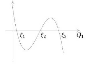
Fig. 2. The graph of Ф 1 ( Q 1 ). The case A 2 <  0.

Рис. 2. График Ф 1 ( Q 1 ). Случай A 2 <  0.

Then we derive

т + c 3 =

-

^δ l 1 ¹

φ 1

dφ

1 - k 2 sin ² ф

Putting here т = 0 , we find an integration constant c ₃ :

^c 3 ⁼

sign P 0

l ₁

_φ 0₁ /

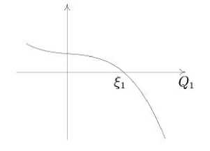
Fig. 1. The graph of Ф 1 ( Q 1 ). The case A 2 <  0.

Рис. 1. График Ф 1 ( Q 1 ). Случай A 2 <  0.

dφ

^/1 - k 2 sin ² ф

ф 0 = 2 arctan a --—

1 _a

Check that k ² <  1 . As z ² + bz + c has no real roots, we have b ² - 4 c <  0 . Therefore,

The case i _A = 1 . Suppose that Ф ₁ has one real root £ ₁ , and that Q 1 G (0 , £ ₁ ) (Fig. 1). Let’s write the integral (36) in the form

Q 1

dz

p( £ 1 - z )( z 2 + bz + c ) ’

( £ 1 + b X 2 < £ 1 + b£ 1 + c = a ² ^ I ^{£ 1 + b/ 2} 1 <  1 .

2 a

Hence, |k ₁ 1 <  1 . Reversing the integral (44) derived above, we come to the function

Q ₁ = £ ₁ + a -

2 a

1 + cn( 1 1 ( т + c 3 ); k 1 ) .

т + c 3 =

δ 1

- 2 A 2

ξ 1

It is easy to see that for Q ₁ G (0 , £ ₁ ) the denominator cn( u ) + 1 = 0 . Calculating the derivative of Q ₁ , we get S ₁ = - signsn ( 1 ₁ ( т + c 3 ); k ₁ ) . For the variable Q ₂ we

find

Q 2 =

4( £ 1 + a ) ⁺

The case i _A = 2 . Suppose that Ф 1 ( Q 1 ) has three real roots 0 < £ 1 < £ ₂ < £ 3 , and Q 11 e (0 ,£ 1 ) . Let’s write (36) as

Note that

n

l 1 ( τ + c 3 )

du

J 1 + n 1 cn( u ; k 1 )

l 1 c 3

f du

J 1 + n 1 cn( u ; k 1 )

n 1 = 1 +

2 a

£ 1 - a'

T + c 3 =

δ 1

2 ^— 2 A 2

ξ 1

/

Q 1

dz

V^{( £} 1 ^— z ^{)( £} 2 ^— z ^{)( £} 3 ^— z )

n ² — 1

-

c k2 = TT > 0'

4 a£ 1

⁺ Q 2 •

Making the substitution ф = arcsin p( £ 1 — z ) / ( £ ₂ — z ) and reversing the resulting integral, we find

Q 1 = £ 2

—

( £ 2 — £ 1 )

cn ² ( 1 1 ( т + c 3 ); k 1 ) ’

where

Therefore for calculating the integral of (1 + n 1 cn( u ; k 1 )) ^{_ 1} we apply the formula (341.03) [15]

^{k 1} = /

^£ 3 ^{— £} 2

^£ 3 ^{— £} 1 ’

¹ 1 = V ^{— 2} A 2 ^{( £} 3 ^{— £} 1 ) •

u

6 du

J 1 + n cn( u ; k )

1              n ²

= 1—n2 n u'n2-3-k)- ng 11 • n2 = 1, (45)

with

sign P ? c 3 =     1 1

_φ 0₁

^ф=, ₀     1 — k ₁ ² sin ² ф

ф 1 = arcsin ^j

£ 1 — Q 1

£ 2 — Q 1 '

Now we calculate δ 1 . We differentiate Q 1 and use the formula of double argument for elliptic sine. We have

g 1 ( u )

= 2/

n ² — 1 k ² + k ‘ ² n ²

Q 1 = ^{2 1} 1 ^{( £} 3 ^{— £} 2 ^)cn

—,

³ ( u ; k 1 )( — 1) sn( u ; k 1 )dn( u ; k 1 ) =

x

Vk ² + k ‘ ² n ² sn( u ; k ) + Vn ² — 1 dn( u ; k )

Vk ² + k ‘ ² n ² sn( u ; k ) — Vn ² — 1 dn( u ; k )

k ‘ ² = 1 — k ² '

Here we note the elliptic integral of the third kind as

u dv

ⁿ⁽ u,n ^{; k} ) = J 1 — n sn 2 ( v ; k ) '

= —11(£3 —£2)cn 4(u; k 1 )(1—k2sn4(u; k 1))sn(2u; k 1), where the notation u = 11 (T + c3) is introduced for brevity. Therefore,

5 1 = sign Q ‘ 1 = — signsn (2 1 1 ( t + c 3 ); k 1 ) '

Now we find Q ₂

For t 1 we have

^Q 2 = 71^ ⁺ 1 ( £ ² —£ 1 ) [n( ¹ 1 ^{( T +} c 3 ) ^,n 1 ^; k 1 ) ^— 4 £ 2       4 1 1 £ 1 £ 2

0            ^ξ 2

— П( 1 1 c 3 ,n 1 ; k 1 ) + Q 2 , n 1 = — '

ξ 1

t 1 = ^{( £} 1 ⁺ a ) ^{T —}

2 a l1

l 1 ( τ + c 3 )

/

du

1 + cn( u ; k 1 )

—

For the value of physical time, corresponding to the variable Q 1 , we have

—

l 1 c 3

Г du

J 1 + cn( u ; k 1 ) '

The integral of (1 + cn( u ; k 1 )) ¹ is calculated by the formula (341.53) [15]

u

/ dv                _x dn( u ; k )sn( u ; k )

----- ---- = u — E ( u ) ± —^v         J , (46) 1 ± cn( v ; k )                  1 ± cn( u ; k )

where E ( u ) = E ( ф ; k ) is incomplete elliptic integral of the second kind ( ф = am u ) .

l 1 ( τ + c 3 )                  l ₁ c ₃

_t = _{£ +} ^£ 1 ^{— £} 2 ^[ Г ^du _— [ ^du 1

1     2        11    L J cn2(u; k 1)    J cn2(u; k 1 )J ’ where the integral of cn_2(u; k 1) is calculated by thefor-mula (313.02) [15]

u

/  , dv . =^ 6(1 — k 2 ) u—

J cn2(v; k)    1 — k2 v dn(u; k) sn(u; k)

^— E ^{( u} ) +--7—----I '

cn( u ; k )

The case i A = 3 . The polynomial Ф 1 ( Q 1 ) has three real roots ξ ₁ < ξ 2 < ξ 3 , and Q ⁰ ₁ ∈ (max { 0 , £ 2 },£ 3 ) . Let us write (36) as

Q 1

т +

5 1      f              dz

² V- ² A 2 J P⁽ z - ^£ 1 ⁾⁽ z - ^£ 2 ^{)( £} 3 - z ) ξ 3

.

The form

reduction of this integral to the standard

(44) is carried out by the substitution ф =

arcsin ( £ 3 - z ) / ( £ 3 - £ 2 ) . The result of reversion can be presented in the form

Q1 = £3 + (£2 - £3)sn2(1 1(т + c3); k 1), where the following notations are used k 1 = 1 /13--42, 11 = P - 2 A 2 (£ 3 - £ 1), ξ3 - ξ1

where the square trinomial z ² + bz + c >  0 for all z . The coefficients b and c are found by the formulae (43). Applying the substitution

,    1 — cos ф             ~ z = £ 1 + a         , a = V/ £1 + b£ 1 + c

1 + cos ф           ¹

and reversing the resulting integral, we come to the function

2 a

1    1   01 +1+cn( 11( т + c 3); k 1) ’ where k2 = . (1 — £ 1 + b/2 ), 11 = 2p20A2.

2 a

^c 3 ⁼

-

sign P ¹⁰

l ₁

_φ 0₁

Z V.

dφ

,

- k ₁ ² sin ² ф

_φ 0₁

sign P ₁ ⁰

c 3 =     1 1    J

ф ⁰ = arcsin

ξ 3 - Q ⁰

ξ 3 - ξ 2

.

For 5 1 we find 5 1 = — signsn (2 1 1 ( т + c 3 ); k 1 ) . Substitute Q 1 in the formulae for Q 2 and t 1 . We find

Q 2 = -7 c ^{1 n(} l 1 ^{( т +} c 3 ) ,n 1 ; k 1 ) ^—

^{4 1} 1 ^£ 3

— П( 1 1 c 3 ,n 1 ; k 1)] + Q 2 ,

dφ

1 — k2 sin2 ф ф10 = 2 arctan \          .

1 _a

As above, one can show that k ₁ ² <  1 . The resulting function Q 1 ( т ) is unbounded, as it has an infinite number of poles on real straight line, which are found by the formula

11 = £, т + SA-b l1

l 1 ( τ + c 3 )

j sn ² ( u ; k 1 ) du— 0

l 1 c 3

— j sn ² ( u ; k 1 ) du .

The integral of squared elliptic sine is calculated by the formula [15]

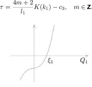
Fig. 3. The graph Ф 1 ( Q 1 ). Case A 2 >  0.

Рис. 3. График Ф 1 ( Q 1 ). Случай A 2 >  0.

u sn2(v; k)dv = ^(u — E(u)). k2

II. Assume further that A 2 >  0 . Now we have Ф 1 ( —го ) <  0 , Ф 1 (+ го ) >  0 , and Ф 1 (0) = с 1 . The qualitatively different cases of the graph Ф 1 ( Q 1 ) are shown in Fig. 3 and 4.

The case i A = 4 . The polynomial Ф 1 ( Q 1 ) has one real root £ 1 and, accordingly, Q 1 (0) >  max { 0 , £ 1 } . The graph of Ф 1 ( Q 1 ) in this case is shown in Fig. 3. Let us write the integral (36) as

т + c 3 =

Q 1

2V2A 2 J

ξ 1

dz

p( z — £ 1 )( z 2 + bz + c ) ,

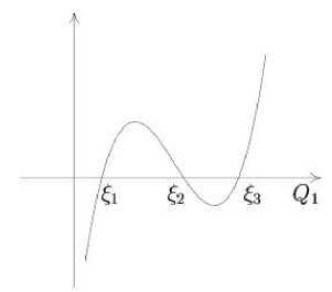
Fig. 4. The graph Ф 1 ( Q 1 ). Case A 2 >  0.

Рис. 4. График Ф 1 ( Q 1 ). Случай A 2 >  0.

Furtherwefind that 5 1 = signsn ( 1 1 ( т + c 3 ); k 1 ) .

For variable Q ₂ we have

Q 2 =

^c 1 ^τ

^{4( £} 1 - a )

-

Reversing (47) and using the inverse substitution, we find the required function

Q1 = £ 1 + (£2 — £ 1)sn2(l 1(т + c3); k 1), where

-

ac ₁

2 1 1 ( £ 2 — a^{1 2}

l 1 ( τ + c 3 )

) ^Z

du

-

l 1 c 3

Z

1 + n 1 cn( u ; k 1 )

du

1 + n i cn( u ; k i )

-

c 3 =

sign P 0

l 1

_φ 0₁

Z V

dφ

^, — k ₁ ² sin ² ф

n ₁ = 1

-

2 a

^£ 1 ⁺ a

.

Note that n ² ₁

n ² ₁

-

7 = 1 +—2

1          n ² ₁

— 1

-

j ⁺ Q 2 ,

ф ⁰ ₁ = arcsin

Q ⁰1

-

ξ 1

.

ξ 2 - ξ 1

One can show that 5 1 = signsn(2 1 1 ( т + c 3 ); k 1 ) . For

Q ₂ we find

( £ — a ) ²

. .     <  0 < k 2 .

4 a£ 1            ¹

Q 2 = 4 lc 1 £ 1 [n( 1 1 ( т + c 3 ) ,n 1 ; k 1 ) —

-

П( 1 1 c з ,n 1 ; k i

ξ 2 n 1 = 1 — ^.

ξ 1

Therefore for calculating the integral of the function (1 + n 1 cn( u ; k 1 )) ^{_ 1} the formula (45) is to be applied with

For the first summand of physical time t in (39) we have

g ¹ = /

1 — n ²

—arctan k ² + k ' ² n ²

k ² + k ' ² n ² sn( u ; k ) #

1 — n ² dn( u ; k ) j ’

-

ξ 2 - ξ 1

t 1 = ^£ 1 ^{т +} —;--- l 1

l 1 ( τ + c 3 )

sn ² ( u ; k ₁ ) du—

k ' ² = 1

-

k ² .

-

If £ 1 = 0 then n 1 = — 1 , and for calculating Q ₂ the formula (46) should be used. For t ₁ we have

l 1 c 3

j sn ² ( u ; k 1 ) duY

Let us consider the case

t 1 = (£ 1 — a)т +    [ l1

l 1 ( τ + c 3 ) ^Z

du

1 + cn( u ; k ₁ )

-

i _A = 6 . Suppose

Q 1 e (max { 0 , £ 3 }, ^ ) . The integral (36) has the form

Q 1

-

l 1 c 3

Z

1 + cn( u ; k 1 ) j .

du

δ 1

^{т +} c 3     2 _x 2 a . J

ξ 3

dz

V ^{( z — £} 1 ^{)( z — £} 2 ^{)( z — £} 3 )

.

Suppose that Ф 1 has three real roots £ 1 < £ 2 < £ 3 . The graph of the function Ф 1 ( Q 1 ) in this case is given in Fig. 4. This case also splits into two subcases: ξ 1 < Q ⁰ ₁ < ξ 2 and ξ 3 < Q ⁰ ₁ .

Using the substitution ф = arcsin 1/( z — £ 3 ) / ( z — £ ₂ ) we transform this integral to the standard form (47). The resulting reversion of the integral in this case is the following

Q 1 = ^£ 2 ⁺

ξ 3 - ξ 2

The case i A

(max { 0 , £ 1 },£ 2 ) . We write (36) as

5 . Suppose that Q 1 e

cn ² ( 1 1 ( т + c 3 ); k 1 ) ’

where

Q 1

δ1   Z т + c3  2V2A2 /

ξ 1

dz

k 1

=

ξ 2 - ξ 1 ξ 3 - ξ 1 ^,

l 1 = p^{2 A} 2 ^{( £} 3 ^{— £} 1 ) ,

V ^{( z — £} 1 ^{)( z — £} 2 ^{)( z — £} 3 )

.

We apply the substitution ф = arcsin V (z — £ 1) / (£2 — £ 1) to this integral and use the notations k 1 = 1 /^2--7i, 11 = P2 A 2( £ 3 — £ 1).

ξ 3 - ξ 1

Then our integral has the standard form

sign P ₁ ^{0 c 3} = "IT”

φ ⁰ ₁

Z q

dφ

^, — k ₁ ² sin ² ф

ф ⁰ ₁ = arcsin

Q ⁰1

Q ⁰1

-

-

ξ 3 ξ 2 ^.

φ 1

δ1 Z т+c3 =l10 V

dφ

Now the function Q 1 ( т ) has an infinite number of poles of the second order, hence it is unbounded. The poles are found by the formula

— k ₁ ² sin ² ф

.

2 m + 1

т = --;---

l 1

K ( k 1 ) — c 3 , m e Z .

Further we find the values δ 1 , Q 2 , t 1

5 1 = signsn (2 1 1 ( т + c 3 ); k 1 ) ,

Q 2 = c r + c S       [n( 1 1 ( т + c 3 ) ,n 1 ; k 1 ) -

^{4 S} 2       ^{4 1} 1 S 2 S 3 ^L

ξ ₂

- П( 1 1 c 3 ,n 1 ; k 1 ) + Q 2 , n 1 = —,

ξ 3

l 1 ( τ + c 3 )

Z _du

J    cn ² ( u ; k 1 )

-

l 1 c 3

Z _du

J cn ² ( u ; k 1 ) ’

An inversion of the integral (38) is fulfilled in a similar way. This integral and the function Ф ₂ differ only by notations from the integral (36) and the function Ф 1 . Therefore, after some evident renaming, we find the expressions for Q 3 , Q 4 , and t 2 . We number these cases sequentially by the parameter i B . Then we have:

i B = 1 о B 2 <  0 , n 2 ,П 3 € C , 0 ⁰ 1 ( Q 3 is bounded ) .

i B = 2 о B 2 <  0 , 0 < Q 3 < n 1 < n 2 < П 3 ( Q 3 is bounded ) .

i B = 3 о  B 2 <  0 , n 1 < П 2 < Q 3 < П 3

( Q ₃ is bounded ) .

i B = 4 о B 2 >  0 , n 2 ,n 3 € C , П 1 < Q 3

( Q 3 is unbounded ) .

i B = 5 о B 2 >  0 , n 1 < Q 3 < П 2 < П 3

( Q 3 is bounded ) .

i B = 6 о B 2 >  0 , n 1 < n 2 < n 3 < Q ⁰

( Q ₃ is unbounded ) .

The study above yield the following theorem.

Theorem 3. The motion of the particle is bounded if and only if at the initial moment both variables Q 1 and Q 3 are restricted on the right by the roots of the polynomials Ф 1 and Ф ₂ , correspondingly.

Now we give a definition of retaining potential, introduced in [14].

Definition 1. A potential is named as retaining , if for arbitrary initial conditions the motion of a particle in a perturbed field corresponding to this potential is bounded.

Thus, potential (28), where G 1 , G 2 are defined by the formulae (40), (41) for A ₂ <  0 and B ₂ <  0 , is retaining. Generally, the formulae (36), (38) are not elliptic integrals, and we cannot present a solution in explicit form. Nevertheless, the above-stated qualitative result remains true [16].

4. Numerical examples and analysis of motions

Example 1. Initial values of coordinates and velocities of a particle:

x1 = 8200 km, x2 = 0 km, x3 = 6000 km, x2 = 8.6 km/s, x 1 = x3 = 0 km/s,

( v _cir к 6 . 26 km/s , v par к 8 . 86 km/s ) .

In an unperturbed case these values define an elliptic motion.

Parameters of potential are as follows:

A - 1 = 0 . 004 km ⁴ /s ² , A 1 = 0 . 06 km ² /s ² ,

A ₂ = 0 . 2 • 10 ^{- 7} km /s ² , B - 1 = 0 . 0001 km ⁴ /s ² ,

B 1 = 0 . 008 km ² /s ² , B ₂ = - 0 . 3 • 10 ^{- 4} km /s ² .

Coordinates of direction vector are b = ( — 1 , 2 , 1) ^T . In the case under consideration the roots of polynomials Ф 1 and Ф ₂ are

S 1 к 1478 , S 2 к 115346 ,

Q “ к 4631 ^ Q 1 € ( S 1 ,S 2 ) , n 2 к 1707 , n 3 к 31031 ,

Q 3 к 5529 ^ Q 3 € ( n 2 ,n 3 ) •

Therefore, the motion is bounded. This is the case i A = 5 , i B = 3 .

The coordinates and velocities have been calculated during a time range, corresponding to two revolutions of the particle around the attracting centre without perturbations, that is т € [0 , 2 T ] , where T is calculated by the formula

I   2"             I x ⁰ 1 ²       ц

^T = ⁿ V ^- h? hk =       ^-t X 0 i.    ⁽⁴⁸⁾

Here h k is the Keplerian energy. Let’s remind that L -transformation doubles the angles at the origin of coordinates.

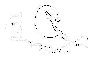
Fig. 5. The case i A = 5, i s = 3.

Рис. 5. Случай i A = 5, i s = 3.

Note that in this example the potential is not retaining. Nevertheless, the motion appears to be bounded. The trajectory of the particle is shown in Fig. 5.

Example 2. Initial values of coordinates and velocities of a particle:

x 1 = 8200 km , x 2 = 0 km , x 3 = 6000 km , x ˙ ₂ = 9 . 9 km/s , x ˙ ₁ = x ˙ 3 = 0 km/s , ( v _cir ≈ 6 . 26 km/s , v _par ≈ 8 . 86 km/s ) .

In unperturbed case the motion belongs to hyperbolic type.

Parameters of potential are as follows:

A - 1 = 0 . 004 km ⁴ /s ² ,  A 1 = 0 . 006 km ² /s ² ,

A 2 = - 0 . 2 · 10 ^{- 7} km /s ² , B - 1 = 0 . 0001 km ⁴ /s ² ,

B 1 = 0 . 008 km ² /s ² , B 2 = - 0 . 3 · 10 ^{- 7} km /s ² .

As A ₂ and B ₂ are negative we have a retaining potential. Coordinates of direction vector are b = (1 , 2 , - 1) ^T . The roots of polynomials:

ξ 2 ≈ 2126 , ξ 3 ≈ 122192633 ,

Q ⁰1 ≈ 5529 ⇒  Q ⁰1 ∈ ( ξ 2 ,ξ 3 ) ,

η 2 ≈ 1699 , η 3 ≈ 81506371 ,

Q ⁰3 ≈ 4631    ⇒  Q ⁰3 ∈ ( η 2 , η 3 ) .

Therefore, the motion is bounded. This is the case i A = 3 , i B = 3 . The integration is carried out during the time range corresponding approximately to t = 1759 . 74 days. The particle trajectory is shown in Fig. 6.

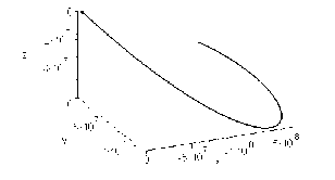
Fig. 6. The case i A = 3, i s = 3.

Рис. 6. Случай i A = 3, i s = 3.

Example 3. Initial values of coordinates and velocities of a particle are as follows:

x 1 = 6000 km , x 2 = 0 km , x 3 = - 8000 km , x ˙ 2 = 7 . 9 km/s , x ˙ 1 = x ˙ 3 = 0 km/s , ( v _cir ≈ 6 . 31 km/s , v _par ≈ 8 . 93 km/s ) .

In an unperturbed case these values define an elliptic motion.

Parameters of a potential are as follows:

A _{- 1} = 0 . 04 km ⁴ /s ² , A ₁ = 0 . 03 km ² /s ² , A 2 = - 0 . 2 · 10 ^{- 5} km /s ² ,  B - 1 = 0 . 1 · 10 ^{- 4} km ⁴ /s ² ,

B 1 = - 0 . 0003 km ² /s ² , B 2 = 0 . 3 · 10 ^{- 4} km /s ² .

Here the potential is not retaining. Coordinates of direction vector are b = (1 , 1 , 1) ^T . The roots of polynomials are as follows:

ξ 2 ≈ 2686 , ξ 3 ≈ 20699 ,

Q ⁰1 ≈ 4423 ⇒  Q ⁰1 ∈ ( ξ 2 ,ξ 3 ) ,

η 1 ≈ 3256 , η 2 , η 3 ∈ C , Q ⁰ ₃ ≈ 5577 ⇒  Q ⁰ ₃ > η 1 .

Therefore, the motion is unbounded. This is the case i A = 3 , i B = 4 .

The integration is carried during the time range corresponding approximately to t = 3 . 23 days. The particle trajectory is shown in fig. 7.

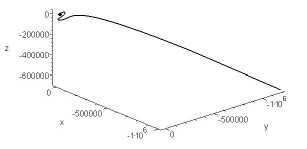
Fig. 7. The case i_A = 3, i_s = 4.

Рис. 7. Случай i A = 3, i s = 4.

In the case of unbounded motion, to define the integration interval firstly one has to find the nearest pole of Q 1 ( τ ) and/or Q 3 ( τ ) in the direction of ascending τ . Suppose this nearest pole is at τ = τ ₁ . Then we choose a small positive value ε and divide the segment [0 , τ 1 -ε ] into N equal subsegments. The value N is to be selected from practical reasons. The orbit should be visually a smooth curve. In our examples the value N = 100 was used. After that, the calculations by the formulae derived above are carried out in equidistant nodes.

The following example demonstrates an application of our formulae for testing a numerical integration method. The original system of motion equations (30) is considered. The Runge-Kutta-Fehlberg method of the eighth order with automatic choice of integration step is tested. The step is chosen by a method of the seventh order. The corresponding pair of programs, implemented in FORTRAN, is below noted as RK F 8(7) . Integration of equations (30) was performed by RK F 8(7) with relative local error of the method ε = 10 ^{- 13} , and all calculations were carried out with double precision (real*8). The gravity parameter and the units of measurement are the same as above. A hypothetical particle is considered, repeatedly encountering the attracting centre. The trajectory obtained by explicit formulae is taken to be standard (reference). Its coordinates have been obtained using Maple with 32 digits (in FORTRAN this corresponds to quadruple precision (real*16)).

Example 4. Initial values of coordinates and velocities of a particle are as follows:

x 1 = 7000 km , x 2 = 0 km , x 3 = 6000 km ,

Estimation of the precision of numerical integration

Оценка точности численного интегрирования

Table 1

Таблица 1

n	t (day)	5H x 10 - 12	5x 1 x 10 12	5x 2 x 10 12	5x 3 x 10 12	Sr x 10 12
1	.3382444	1	0.2	1	1	0.4
10	4.9080991	2	6	12	213	10
50	24.1940313	41	729	104	1667	108
100	48.4322508	53	4399798	523748	95154	330606
500	242.7821163	294	77898	31418	151259	77206
1000	485.2955201	556	554500	332688	1067003	330900

x ˙ ₂ = 7 . 9 km/s , x ˙ ₁ = x ˙ ₃ = 0 km/s ,

( v cir и 6 . 58 km/s , v par и 9 . 30 km/s ) .

In an unperturbed case we have an elliptic motion.

Parameters of retaining potential are as follows: A - 1 = 0 . 1 km ⁴ /s ² , A 1 = — 0 . 02 km ² /s ² , A ₂ = — 0 . 2 • 10 - ⁵ km /s ² , B - 1 = — 0 . 004 km ⁴ /s ² , B 1 = — 0 . 001 km ² /s ² , B 2 = — 0 . 001 km /s ² .

Coordinates of direction vector are b = ( — 1 , — 3 , 1) T .

The roots of polynomials Φ ₁ and Φ ₂ are as follows:

£ 2 и 764 , £ з и 58639 ,

Q о » 4459 ^ Q 1 e ( £ 2 ,e 3 ) , П 2 и 504 , n 3 и 7209 ,

Q 3 и 4761 ^ Q 3 e ( n 2 ,n 3 ) .

Therefore, the motion is bounded. The case i A = 3 , i _B = 3 .

The calculations were carried out during the time ranges corresponding to 1, 10, 50, 100, 500, and 1000 revolutions of the particle around attracting centre without perturbations. The trajectory of the particle for three revolutions is shown in Fig. 8.

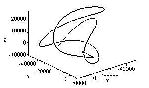
Fig. 8. The case i_A = 3, i_B = 3. The motion is bounded.

Рис. 8. Случай i A = 3, i B = 3. Движение ограничено.

Table 1 contains the values, near the end of the integration interval, of the relative error for the energy constant δH , the coordinates of particle position vector x _i , and its absolute value r

δH =

H ⁰ — h |

|h I

SX i = x-^ c ¹, i =1 , 2 , 3 , ^|x i ^|

^| _r ^— r c ¹ δr =

r where H0 is the value at the initial moment, H at an arbitrary moment; xic, rc are the values found by exact formulae. In the second column the intervals of physical time t (in days) are given, for which numerical integration of system (30) was carried out.

From these data we can see that if the integration interval increases, the relative errors of H and x 3 do not decrease. For coordinates x ₁ , x ₂ , and absolute value r , with n = 100 , these errors increase, then they diminish, and then increase again.

The numerical examples show efficiency of the formulae we obtained. Besides, the theorem 3 allows to determine, given the initial position and velocity of a particle, whether its motion is bounded or unbounded.

Conclusion

In this paper we consider three sorts of coordinates (regular q -coordinates, bipolar coordinates, spherical coordinates). For each of the systems, the forms of potentials admitting complete separation of variables are given. Thus, the original equations for such potentials allow integration “in the sense of Sundman”. In a similar way one can build, for regular q -coordinates, other coordinate systems for which Hamiltonian has orthogonal form, and with the use of Stackel theorem build potentials allowing the abovementioned integrability.

Application of these potentials is a separate and independent problem. These potentials are of practical importance, which approximate some real forces.

The author is grateful to professor A.Zhubr for useful comments and discussions.