Predicting Financial Prices of Stock Market using Recurrent Convolutional Neural Networks

Financial time series analysis is the core value in the scope of various research areas, and gained much attention in several engineering problems. The time series data is relates to calculating useful features and pattern features of sequence data. During a period of time, the observations of time series data is collected and taken by sequentially. A time series is a collection of observations of data items taken sequentially during a period of time. Predicting financial time series is greatly complex, due to the substantially the most highly-noise characteristics and the strong form of market effectiveness, accepted through the general. In recent years, Deep Learning models have been applied in many time series financial applications, in particular ” automatic time series predictions and computer vision [1]. These approaches have also attained and enhanced the performance in financial sequence predictions, when compared to conventional machine learning algorithms. “ For illustration, some researches on investment market abnormalities have illustrated more than 130 include deviations efficiently overcome the market relying on return predictive signals. These signals are used as features (input) in order to predict particular financial return as the targets (output) by using deep learning approaches. However ” due to the powerful feature learning ability, auto encoder (AE), convolutional neural network (CNN) and recurrent neural network (RNN) become the famous approaches and have been used in the financial sequence prediction tasks [2].

Aloysius [8] Proposed a statistical arbitrage technique based on deep restrictive contingent portfolio categories apply random forests (RFs). Moreover to adjust the return of U.S on per month CRSP stock world between the 1967 to 2011

In this research, we follow the combination way and design two networks architecture: Our contributions are summarized as follows: First, we concentrate on revising the standard gated recurrent unit (GRU) model, which greatly addresses vanishing gradient and exploding issue of standard RNNs over the gating mechanism and make the ordinary architecture and retaining the impact of LSTM (is a well-known variant of traditional RNNs). Second, we proposed to combine GRU with CNN architecture to identify financial marketing predictions based on the return predictive signals. Third, we also trained our model with attention mechanism (GRU-CNN) and compare the performance with the traditional deep learning models. Fourth, experiments show that our enhance GRU-CNN model achieves better predictions performance than previous traditional methods. In statistics and economically, ” the existing GRU-based model obtains good accuracies and more returns. But the proposed GRU-CNN model performs slightly better than GRU-based model.

The rest of this paper is organized as follows: the related work is introduced in section II, while traditional deep learning models are discussed in Section III. The problem identification in standard RNN is given in section IV. The detail of the proposed GRU-CNN architecture and flowchart are described in section V. The experimental setup is provided in section VI. Results and discussion are illustrated in section VII. Finally, this work is summarized conclusion in section 5.

2.    Related Works

The authors [17] worked on S&P 500 volatility based on the standard LSTM model by applying the Google stock domestic trends as an indicator of the market volatility. LSTM is a powerful model to addresses the vanishing gradient issues which are common issues in the training of traditional RNN. Dixon [18] proposed deep neural network to trained model using multiple financial instruments for prediction of market trends and also classify the future trend as either positive, flat or negative. “ X Ding et al in [16] conducted a research on financial time series prediction with combination of Natural language processing (NLP). For stock market prediction in [19], authors applied two machine learning approaches such as Least Square Support Vector Machine (LSSVM) and Particle Swarm Optimization (PSO). The dataset consists of combined all symbols with training feature sets, each engineered features and price differences encoded by 9889. The deep learning models usually contain of five fully connected layers and the model is show the prediction of instrument’s trend however ignore operation costs.

3.    Deep Models

Deep learning techniques were derived from artificial neural networks and nowadays it is a predominant arena of machine learning and has achieved an outstanding performance in several research areas, like as time series prediction, computer vision and NLP. However, its practicality deep learning becomes more prevalent for several researchers to do research works.

• 3.1.    Convolutional neural network

• 3.2.    Recurrent neural network

  A Recurrent Neural Networks (RNNs) is a kind of supervised neural networks that was initially introduced by Hopfield in 1983. It has connections between the nodes form a bidirectional cycle, and they perform well on the sequential tasks. The RNN approach performs excellently on sequential problem specially extracting temporal information in the loop. RNN is capable to compute a sequential of random dimension through recursively using a transition function to its internal hidden state vector h t of the sequential inputs. The structure of an RNN is presented in Fig.2. When sequence inputs are required as X = [x 1 , x 2 ... x t ... x T ] of dimension T, O t is a output vector, and are present the hidden state at the time t of the RNN are summarized the following equations:

A convolutional neural network (CNNs) are one of the most widely biologically inventive kind of forward deep neural network (DNN) that has recently achieved popularity due to its achievement in many fields of research such as classification problems and financial time series predictions [20]. CNNs architecture is mainly contained on three layers are included convolution layer, pooling layer and fully connected layer. It demonstrates to be capable to extracts high level features concept from sequential representation of input data, and then combines these features by the subsequent layer in order to achieve higher order features. Each single layer of a CNN uses a differentiable function in order to transfer information from one volume of activations to the next. Convolutional layer is a fundamental layer of a CNN and involved most of the computation process [21]. Training iterations (epochs) uses gradient decent to train the convolutional layer and model parameters are combined by a Rectified Linear Units (ReLU) layer to support non-linear function [8]. The pooling or subsampling layers of CNNs extracts the values of their filter size during the training stage based on the tasks. The schematic presentation of CNN is shown in Fig.1.

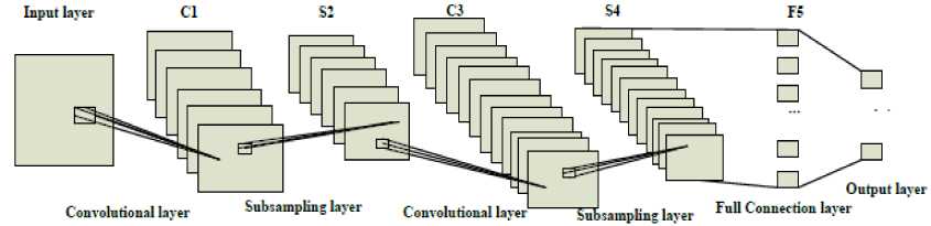
Fig.1. A schematic presentation of CNN

A further kind of layer, the max pooling layer, is commonly used in CNNs. It works on data to compresses and makes smooth data. Max-layer selects the maximum value of the receptive field and produces data invariant to small translational changes [22]. Consequently, ” generate three CNNs layers to manage various data prediction due to their variances in sizes. When apply subsampling layers and for final output using fully connected layer. This structure of CNN enables the model to acquire filters that is capable to identify particular features in the input data. Recently advance in CNNs for sequential time series prediction included by [23] where the researcher have to proposed an undecimated convolutional networks for time series modelling based on the un-decimated wavelet transform. “ Instinctively, the concept of using CNNs to time series prediction would be to determine filters that show the convinced recurrence features in the series and apply to predict the future values. Due to the layered architecture of CNNs, they able to perform better on noisy data, by removal noise in each subsequently layer and capturing only the useful information [24].

O = awx + их ; ) (1)

a , = ^Wx. + U o h , + 1 )

O t = [O , : O , ]

where W g R O ^X O x is refer the weights matrix connection between input layer to hidden layer, and hidden layers weights matrix are presented by U_o g R O h ^X O h . о is the sigmoid activation function and W_x , U_o , are parameters of the existing RNN.

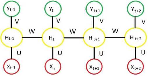
Fig.2. Standard architecture of RNNs ht refer to the hidden state at time-step t is computed by Ot and the previous hidden state ht-1. Whereas the RNN is an excellent model for handling sequential problems, it is hard to train with the gradient descent method and suffer from vanishing and exploding gradient (explosion) issue. In contrast, the variants of RNN have been introduced to solve this issue, such as Gated Recurrent Unit (GRU), it avoids overfitting, as well as saves training time. Therefore, we adopted GRU in our technique.

• 3.3.    GRU based model

The gated recurrent unit GRU is comparatively recent development introduced by Cho et al [25], that addresses the common issues of long term dependencies which can leads to poor gradients for larger traditional RNN networks. The GRU is a simplified variation of the LSTM and it has gating mechanism that controls the flow of information inside the unit without having a separate memory cells. GRU is much simpler to calculate because it has two gates called update gate and reset gate are applied to appropriately extract dependencies through various time scales: the reset gate r t , decide control information from the previous time step is kept in the candidate hidden state; another is the update gate z t , which decides to handle previous information through away and how much information from the candidate hidden state is added.

P(y=0|x)

Softmax

P(y=1|x)

P(y=2|x)

Output layer

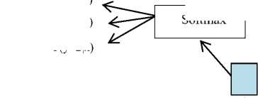
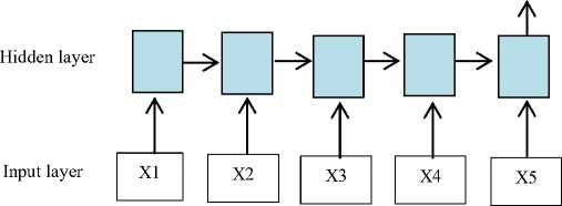
Fig.3. Structure of GRU-based model.

The input layer of the model is composed of multiple neurons is presented in Fig. 3, the number of neurons is decided by the dimension of the features space. The design of GRU combines forget and input gates into a single unit named “update gate”, and has an additional “reset gate” that handle the flow of information inside the unit without having an individual memory cells [26]. GRU also demonstrates the superior ability of modeling to capture long-term dependencies among the sequential elements and have to gain progressive popularity.

To calculated these gates for time step t by the following equations:

Update gate:

z_t = G (W .[ h_t - 1 , x_t ] + b )                                              (4)

Reset gate:

r_t = G g (W r .[ h - 1 , x ] + b_r )                                              (5)

Candidate state h = tanh(W. [rt * ht_ 1, xt ] + b^ )                                              (6)

Final output h = (1 -z,)*h-1 + zt *ht                                             (7)

where W^z, W^r, and W^x are the weights of update gate, reset gate, and candidate state accordingly, and the biases of these gates are presented by b z , b^r and - b^h . Equations (4) and (5) are applied to calculate the update and reset gates respectively. h_t ” is the candidate hidden state function defined in (6) which is applied to calculate the hidden activation h given by (7)

• 4.    Problem Identification

  Define Recurrent neural networks (RNNs) are prevalent architecture that can perform well on sequence dataset. The concept behind RNNs is to store similar portions of the inputs and apply this information to predicting the output in the future. Therefore, the RNNs are most suitable for time series predictions. However, unfortunately the RNNs often suffer from the vanishing gradient and exploding issues, which performance in unsuccessful to capture long-term dependencies. It makes the training of RNN difficult, in two ways: firstly, it cannot process very long sequences if using hyperbolic tanh activation function and secondly, if network is unfolded based on the several time steps which some of the RNN weights initiates to convert too large or too small due to gradient and exploding issues. Based on observation, to avoid this issue, two variations of RNNs have been introduced, which applies a gating mechanism to handle these issues. A latest kind of RNNs called gated recurrent unit (GRU) proposed by Cho et al in 2014 [25] that tackle this kind of issue.

• 5.    GRU-CNN Proposed Architecture

Based on the ordinary implementation, to calculate units composed by gates in order to reduce the error in the block, due to replace the hidden layer by in complex block, constructing known as error carrousel. Financial sequence predictions contract with the capturing of the basic features to evaluate and the temporary dynamics prediction of financial assets. Due to the inherent uncertainly and non-analytic structure the prior works in this field concentrates on technical analysis, the task showed to be challenging in the prediction of financial markets inherent uncertainty and non-analytic architecture, where classical linear statistical approaches are including the ARIMA model and statistical machine learning (ML) approaches have been extensively used time series tasks [18].

In this section, we further investigate to introduce integrated design of the recurrent convolutional neural network model for the financial prediction of trading signals is presented in Fig. 4. GRU is ability of learning some dependencies which efficiently remove the vanishing gradient issue. GRU is basically similar to an LSTM controls the information inside the unit but it has no output gate. The activation h t is referring to the final output of GRU at time t among the previous state h - and the candidate state h_t :”

ht = (1 -z)*ht-1 + z *ht(8)

The update gate z t help the model to control how much of the previous information updates its activation.

z = Sigm (Wxzxt + Uzh-1 )

The reset gate r t determine how much of the previous information to ignored its activation.

r = Sigm (WxrXt + Uhzh,-1)(

The candidate activation h_t is computed similarly to the update gate:

ht = tanh (Whxt + Uhh (rt* ht-1))(11)

We replace hyperbolic tangent activation function ( tanh ) with ( Relu ) in equation (11) the new equation is:

ht = Relu (WxhXt + Uhh(rt* ht-1))(12)

where Sigm is a sigmoid activation and ∗ is refer an element-wise multiplication. Reset gate allows the unit of ignore previous information, when it is very close to zero or off (“rt == 0). The reset gate is computed through the following equation:

r t = Sigm (W xr x t + U hz h t - 1 )

Update gate z t updates the following information sending by previous activation with time step t and pass to the next step. On the other hand, reset gate r t control the short-term dependencies and long-term dependencies has controlled by update gates z t in the GRU model. In this paper, we addresses the limitation of the above models, we proposed a Recurrent Convolutional Neural Network and it apply for the task of financial sequence perdition. We construct the time series prediction model (GRU-CNN financial sequence prediction model) with GRU and CNN deep learning model. It mainly includes five parts of layers namely, input layer, convolutional layer, GRU layer, pooling layer and finally fully connected layer are presented in Fig. 4.

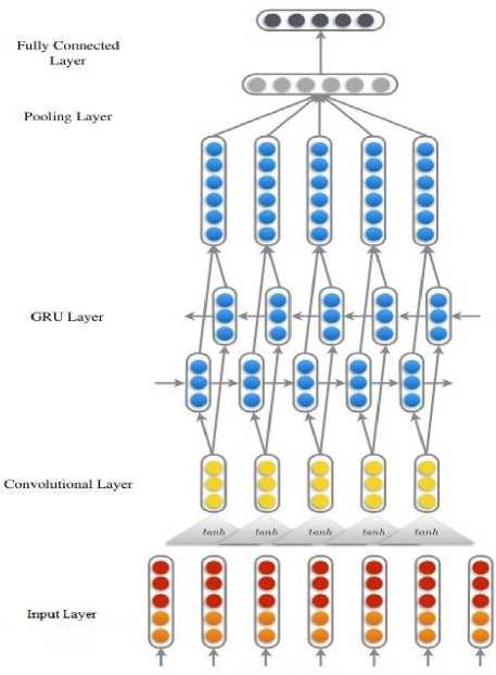
Fig.4. Proposed GRU-CNN architecture

In Fig.4 illustration, the first layer is input layer for preliminary study of data values. In the first layer of CNN, the original values are observed into a high dimensional space, so that the original values prediction can be distinguished better. The 2^nd layer of CNN is convolutional layer that perform convolution operation can extract this information by combining high dimension features in a fixed window. Provided the sequential inputs representation x = (x 1 , x 2 ,...,x n ) and a context window length k, concatenation of sequential prediction in this window length can be determined as X j = [x j ^T,...,x j+k-1 ^T ]^T , and the representation of this sequential prediction sample can be reformatted as X = (X 1 ,...,X n-k+1 ). Provided a weight matrices of the convolutional filters W^conv and a linear bias b , the local features representation are calculated:

C = tanh(W^conv . X, + b )

where “Wconv∈Rdc×dxk, b∈Rdc, and tanh denotes the hyperbolic tangent function. Generally, the convolutional layer output generated from Eq. (14) is further processed as inputs to the GRU layers passing through the reset gate and update gate based on the Eq. (9) and Eq. (10) to perform the most considerable prediction. However, these sequential predictions are independent. GRU has the capability to handle this weakness by applying a gating architecture to extract short-term and long-term dependencies. Therefore, in this research, a GRU layer is built on top of the convolutional layer to continue the financial sequential prediction task. Note that sequence financial prediction using fully connected layer is perform similar as a softmax layer. The difference between fully connected layer and softmax is in only their goals parametrized by all weights matrix W. Softmax layer reduces the cross-entropy or increases the log-likelihood; however to find out the maximum margin among the data points and various classes is efficiently performed by max-pooling layer.

In this research, we concentrate overall performance of the proposed architecture to predict the stock market trading signals. Fig.5 is presenting the flowchart of the proposed algorithm for predict the trading signals.

In order to train the GRU networks efficiently in this research we developed to apply three basic methods. Initially we set the RMSprop optimizer is derived from rprop, and applied mini-batch in the model training. This technique is usually select for RNNs approaches. Secondly, the dropout regularization applied in the hidden layers in order to avoid overfitting. According to a certain probability, the neural network units discarded from the network in the training procedure. Thirdly, we have to use early stopping criteria in this research to achieve the same purpose as a further mechanism. Moreover, the dataset is splitted according to a specific ratio into training set and validation set. The former set is applied for training, while obtained test results by verification set (e.g., every 5-epoch is considered for test).

The best amount of the post-sample data between the samples is verified as 20%, the data divided into training and validation set according to the following ratio of 4:1. We set 10000 epochs in the training process and the maximum early stopping duration to 10. By this means, we provided a particular explanation of the proposed GRU-CNN model as follow:

Input layer with 250 time-steps consisting one feature.

The hidden layer of GRU consists of 27 hidden neurons and 0.5 selected as dropout rate.

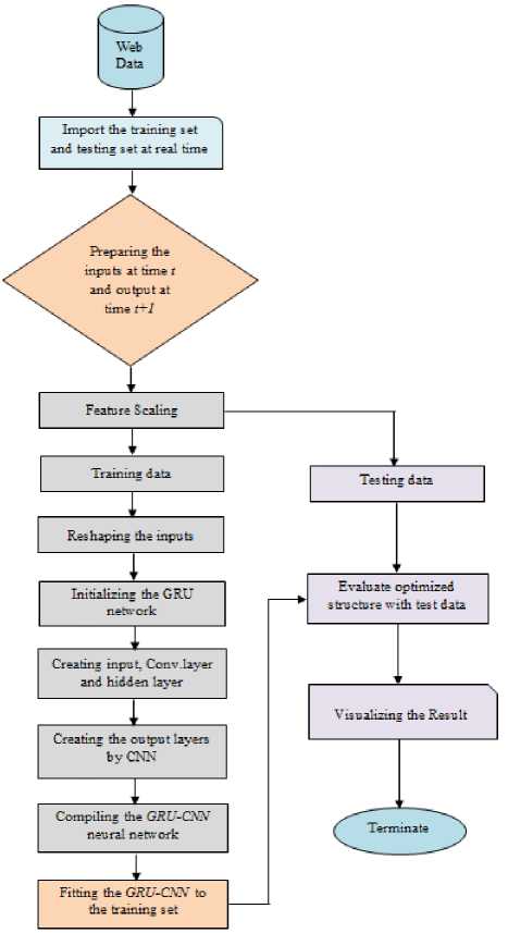
Fig.5. Flowchart of model for predicting the stock market trading signals

• 5.1.    Deep GRU-CNN and Benchmark models

6.    Experimental Setup

• 6.1.    Datasets & Software

  The first step in this research is Data exploration. In this research the database are contains specific representative in financial marketing predictions by Asia, Europe and the Americas [27] publicly available and downloaded through Yahoo Finance for the period between 2008 and 2016. In this research, we train and test proposed and comparative models on three financial marketing data are namely, HSI, the DAX and the S&P 500 Index as the raw data. Because the main focus of these experiments are completely demonstration financial market and without the instability of separate stocks, for the trading probability technique the high-liquidity are selected as a subsets of the stock market is a most actual test set for computed probability. Statistics summary of experimental datasets is explained in Table 1.

• 6.2.    Generation of training and trading sets

  The study analysis on the daily basis of data between “2008 to 2016 are collected the training and trading period is determined training-trading sets. The previous set about 750 days, almost three years” for sample training. The latter used for out-of-sample trading is set to “250 days, equivalent to one year. With this structure, we have offered lot of training samples for the proposed architecture in section 3 to be evaluated. Based on this, the sliding-window approach is referred; the training-trading set is move forward by a length of 250 days. Furthermore, the 24 batches are not overlapped with each other looping over the entire dataset among 2008 and 2016 as given in Table 1.

7.    Results and Discussion

In this section, for the traditional GRU and the proposed GRU-CNN model have mention above, we optimize to combined recurrent neural networks (RNNs) to present the advantage of the existing GRU network, and evaluates the performance of conventional CNN. Specially, the input features (standardized returns) and the output targets are general in the similar method as signified in the previous subsection.

In this paper, a typically organized a comparative study of deep learning approaches with our proposed GRU-CNN model in order to evaluate the performance and advantage of the model. The input layer consists of 246 neurons according to the input features, and three fully connected nodes are selected in the output layer. For learning high statistical features, we have to select three hidden layers, each layer consist number of several neurons from the first layer to the third layer is 1, 2 and 3 individually. The model training simulated is executed 5 times for each combination of momentum. We applied rectified linear unit (Lelu) as the activation function and learning rate 0.001 as well as 0.5 set as a dropout. Based on the gird search approach these parameters are optimizing to avoid overfitting and under-fitting. For the purpose of validation, we apply k-fold cross validation with k=5 in the data partition. By comparative analysis of the proposed model with different state-of-the-art approaches, we proved that the proposed GRU-based approaches with CNN are capable to achieve more significant results than other state-of-the-art approaches through more complicated and intensive computations.

Table 1. Summary of experimental datasets.

Index	Time period	Sample size
HIS	18/05/2008 – 14/05/2016	6640
DAX	18/05/2008 – 11/05/2016	6812
S&P 500	22/05/2008 – 10/05/2016	6719

Data preprocessing and manipulate are carried out in Python 3.6 and anaconda depending on the packages scipy, sklearn, numpy and pandas. For quick implementation of the proposed model and traditional deep learning models are implemented, an effective open source software library for numerically computational using data flow graphs in which permits an ordinary and rapid develop. All the simulation works were carried out on Intel Core i7-3770CPU on a Windows PC with @3.40 GHz, and 4GB RAM ” machine.

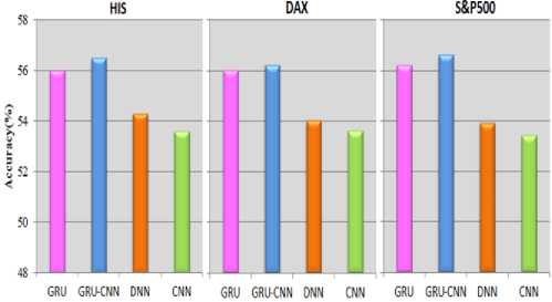
For every index, accuracy that has been used as an evaluation metric for trading sets to evaluate the performance of proposed GRU-CNN model and comparative approaches, for the proportion of accurate classification it is an important metric has been achieved by computing in deep learning.

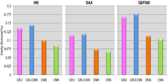
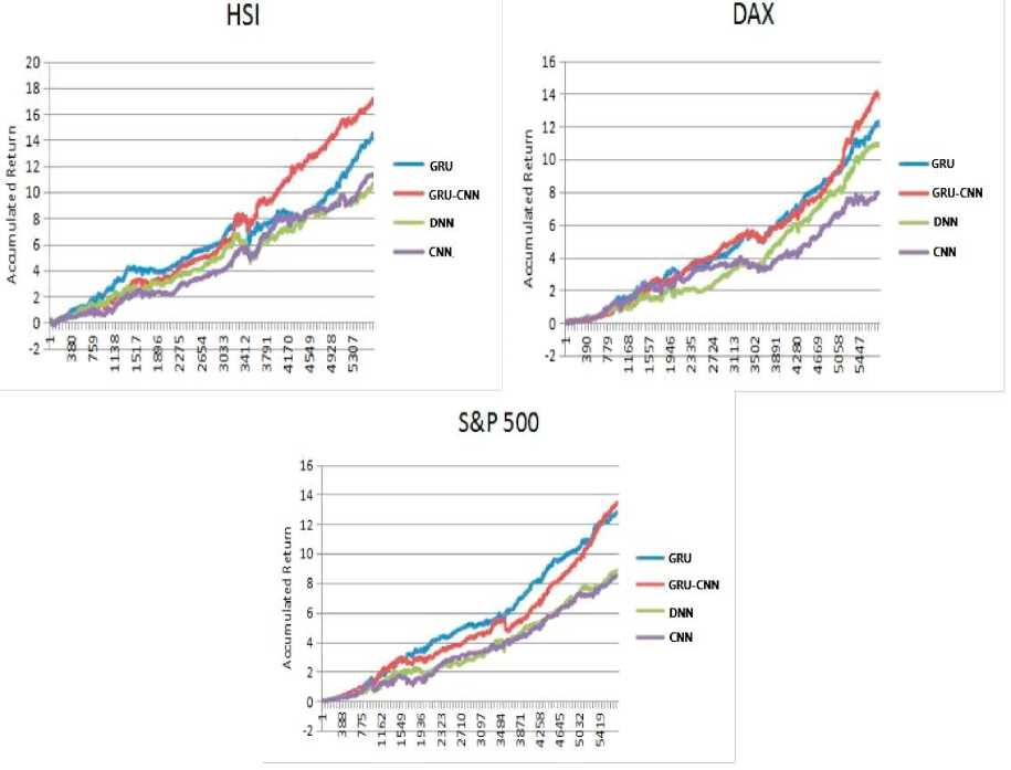
In addition, we evaluated the efficiency and effectiveness of the proposed model by daily mean returns and cumulative returns of the trading periods. The formulas calculate the daily mean return and cumulative returns as a follows:

Daily Returns [%] = —---— P. -i * 1

P - P

Accumulative Returns = [ R ] = current ----initial-                                  (16)

c             Pinitial where pt is a current price, pt-1 is a previous price and ∗ denotes as a multiplication element.

According to the following trends we reported the accuracies of various deep learning approaches are presented in Fig.6. The performance of the standard GRU model and the proposed GRU-CNN model in the term of accuracy are always greater than 55% on the stock indexes dataset, it is significant benchmark for a dollar neutral scheme, its presents that our proposed approach for analyzing the prediction tasks on financial time series. Regardless this kind of dataset, the proposed GRU-CNN model performs excellent as compared to other state-of-the-art approaches. Experimental results has presented that the proposed model achieved 56.2% results in term of daily returns and Accumulative returns, while GRU is obtain 55.8% , DNN is achieve 53.9%, and 53.5% is achieved by CNN for S&P 500. In this way, a same condition is occur in other two indexes, the proposed GRU-CNN model have achieved excellent performance, with the exclusion of the “ DAX are presented in Fig.7 and Fig.8.

8.    Conclusion

In this paper, we present combination based architecture of “ CNN with RNN for financial sequence predictions. We applied GRU network and replace its traditional output layer with CNN to predict the operation signal on the three stock indexes HIS, the DAX and the S&P 500, among May 1990 and August 2016. The proposed model is showed effectiveness and higher value through the experimental results detailed. Based on the proposed mechanism, the GRUbased architecture is used to capture meaningful information from a vast array of financial time-series data has been presented to be effectively, and for the final output that CNN outperform to usage fully connected layer. Our proposed model achieved superior performance in the term of accuracy, daily mean returns, and accumulative returns as compared to others traditional deep learning models namely GRU, DNN, and CNN. Furthermore, ” it will be remarkable to observe future work on implementing proposed model for further time series applications such as weather forecasting, earthquake prediction and signal processing.

Acknowledgments

The authors would like to thank the Ministry of Higher Education Malaysia (MOHE) and Universiti Tun Hussein Onn Malaysia for funding this research activity under the Fundamental Research Grant Scheme (FRGS/1/2017/ICT02/UTHM/02/5), vote no. 1641.