Prediction of Missing Associations Using Rough Computing and Bayesian Classification

Published Online October 2012 in MECS

The amount of data collected across a wide variety of fields today far exceeds our ability to reduce and analyze without the use of automated analysis techniques. There is much information hidden in the accumulated voluminous data. It is very hard to obtain this information. So, it is essential for a new generation of computational theories and tools to assist human in extracting knowledge from the rapidly growing voluminous digital data. Knowledge discovery in databases (KDD) is the field that has evolved into an important and active area of research because of theoretical challenges associated with the problem of discovering intelligent solutions for huge data.

Knowledge discovery and data mining are the two rapidly growing interdisciplinary fields which merge database management, probability theory, statistics, computational intelligence and related areas. The basic aim of all these is to extract useful knowledge and information form voluminous data.

The process of knowledge discovery in databases and information retrieval appear deceptively simple from the perspective view of the terminological definition [1]. Knowledge discovery in databases is defined as “the nontrivial process of identifying valid, novel, potentially useful, and ultimately understandable patterns in data”. It tells that knowledge discovery process consists of several stages: data selection, cleaning of data, enrichment of data, coding, data mining and reporting. However, the data mining phase has become one of the most popular areas of recent research. The closely related process of information retrieval and data mining is defined [2] as “the methods and processes for searching relevant information out of information systems that contain extremely large numbers of documents”. In execution, however, these processes are not simple at all, especially when executed to satisfy specific personal or organizational knowledge management requirements.

The earliest and the most successful technique being used in data mining is the notion of fuzzy sets by Zadeh [3] that captures impreciseness whereas rough sets of Z. Pawlak [4] is another attempt that captures indiscernibility among objects to model imperfect knowledge [5, 6, 7]. There were many other advanced methods such as rough set with similarity, fuzzy rough set, rough set on fuzzy approximation spaces, rough set on intuitionistic fuzzy approximation spaces, dynamic rough set, were discussed by different authors to extract knowledge from the huge amount of data [8,9,10,11,12].

Missing data is a common problem in knowledge discovery, data mining and statistical inference. Several approaches to missing data have been used in developing trained decision systems. Little and Rubin [13, 14] have studied and categorized missing data into three types: missing completely at random, missing at random, and not missing at random. The easiest way to handle missing values is to discard the cases with missing values and do the analysis based only on the complete data. But, the absence of missing associations among attribute values and missing data may have information value to predict the decision.

In this paper, we use two processes such as pre process and post process to predict the decision values for the missing associations in the attribute values. In pre process we use rough set on fuzzy approximation spaces with ordering rules to find the suitable classification of data set, whereas in post process we use Bayesian classification to explore decision values for the missing associations in the attribute values. Rest of the paper is organized as follows: Section 2 presents the basics of rough set on fuzzy approximation space. We present the basic idea of order information system in Section 3. In Section 4, we discuss the Bayesian classification whereas in Section 5 we propose prediction model. In Section 6, an empirical study on cosmetics companies were considered to analyze our proposed model. This is further followed by a conclusion in Section 7.

• II.    Rough Set on Fuzzy Approximation Space

Convergence of information and communication technologies brought a radical change in the field of decision making. It is a well established fact that right decision at right time provides an advantage in decision making. But the real challenge lies in converting huge data collected across various domains into knowledge, and to use this knowledge to make informed business decisions. Classical set has been studied and extended in many directions so as to model business decisions. Later the notion of fuzzy set by Zadeh [3], its generalizations and the notion of rough set by Pawlak [4] were the major research in this direction. The rough set philosophy is based on the concept of indiscernibility relation. The basic idea of rough set is based upon the approximation of sets by pair of sets known as lower approximation and upper approximation with respect to some imprecise information. However, indiscernibility relations in real life situations are relatively rare in practice. Therefore, efforts have been made to make the relations less significant by removing one or more requirements of an indiscernibility relation. A fuzzy relation is an extension of the concept of a relation on any set U . Fuzzy proximity relations on a universal set U are much more general and abundant than equivalence relations. The concept of fuzzy approximation space which depends upon a fuzzy proximity relation defined on a universal set U is a generalization of the concept of knowledge base. Thus, rough sets defined on fuzzy approximation spaces extend the concept of rough sets on knowledge bases as discussed by Acharjya and Tripathy [9].

Let U be a universe. We define a fuzzy relation on U as a fuzzy subset of (U×U). A fuzzy relation R on U is said to be a fuzzy proximity relation if µ (x, x) = 1 for all x∈ U and µ(x, y) = µ(y,x) for x,y ∈U . Let R is a fuzzy proximity relation on U. Then for a given α ∈ [0,1], we say that two elements x and y are α- similar with respect to R if µ(x, y) ≥ α and we write xR y or (x, y) ∈ R . We say that two elements x and y are α - identical with respect to R if either x is α- similar to y or x is transitively α- similar to y with respect to R, i.e., there exists a sequence of elements u ,          u ,u ,   ,u      in     U such that xRαu1, u1Rαu2 , u2Rαu3 ,  , u R y . If x and y are

α 1   1 α 2   2 α 3            n α

α- identical with respect to fuzzy proximity relation R, then we write xR(α) y , where the relation R(α) for each fixed α ∈ [0,1] is an equivalence relation on U. The pair (U, R) is called a fuzzy approximation space. For any α∈ [0,1], we denote by R* , the set of all equivalence classes of   R(α)   . Also we call (U, R(α)), the generated approximation space associated with R and α . Let us consider X⊆ U. Then the rough set on fuzzy approximation space of X in (U, R(α)), is denoted by (X, Xα) , where X is the α- lower approximation of X and Xα is the α- upper approximation of X. We define X and X α as follows:

X _α = ∪ { Y : Y ∈ R _α ^* and Y ⊆ X }                 (1)

X α = ∪ { Y : Y ∈ R ^* and Y ∩ X ≠ φ }             (2)

Then X is said to be α - discernible if and only if X = X α and X is said to be α - rough if and only if X _α ≠ X α .

• 2.1    Almost Indiscernibility Relation

An information system is one that provides all available information and knowledge about the objects under certain consideration. Objects are only perceived or measured by using a finite number of properties. At the same time, it does not consider any semantic relationships between distinct values of a particular attribute [15]. Different values of the same attribute are considered as distinct symbols without any connections, and therefore on simple pattern matching we consider horizontal analyses to a large extent. Hence, in general one uses the trivial equality relation on values of an attribute as discussed in standard rough set theory [4].

However, in many real life applications it is observed that the attribute values are not exactly identical but almost identical [9,  16,  17,  18]. At this point we generalize Pawlak's approach of indiscernibility. Keeping view to this, the almost indiscernibility relation generated in this way is the basis of rough set on fuzzy approximation space as discussed in the previous section [9]. Generalized information table may be viewed as information tables with added semantics. For the problem of predicting missing associations, we introduce order relations on attribute values [19]. However, it is not appropriate in case of attribute values that are almost indiscernible.

Let U be the universe and A be a set of attributes. With each attribute a∈ Awe associate a set of its values V , called the domain of a . The pair S = (U, A) will be called an information system. Let B⊆ A. Forα∈ [0,1], we denote a binary relation R (α) on U defined by xR (α)y if and only if x(a) R(α) y(a) for all a∈ B, where x(a) ∈ V denotes the value of x in a. Obviously, it can be proved that the relation R (α) is an equivalence relation on U. Also, we notice that R (α) is not exactly the indiscernibility relation defined by Pawlak [9]; rather it can be viewed as an almost indiscernibility relation on U. For α = 1 the almost indiscernibility relation, R (α) reduces to the indiscernibility relation. Thus, it generalizes the Pawlak's indiscernibility relation. The family of all equivalence classes of R (α) i.e., the partition generated by B for α ∈ [0,1] , will be denoted by U/R(α) . If (x, y) ∈ R (α) , then we will say that x and y are α - indiscernible. Blocks of the partition U/ R(α) are referred as B - elementary concepts. These are the basic building concepts of our knowledge in the rough set on fuzzy approximation space.

• III.    Order Information System

  Let I = ( U , A , V , f ) be an information system, where U is a finite non-empty set of objects called the universe and A is a non-empty finite set of attributes. For every a ∈ A , V is the set of values that attribute a may take and f : U → V is an information function. A special case of information systems called information table or attribute value table where the columns are labeled by attributes and rows are by objects. Consider the information system given in Table 1. Here, we have A = {3G, Touch screen ( ts ), Screen size ( ss ), Camera resolution ( cr ), Sim ( s ), Price} and V = { Yes , No } . Similarly, we get V = { Yes , No } , V = {1.8'', 2.2'', 4.3'', 2.4'', 3.5'}, V = { Dual , Single } , V = {VGA, 3.2MP, 8MP, 3.2MP, 2MP}, and V = {3500, 13300, 29300, 13000, 30000}.

Table 1:  Information System

Object	3G	Touch screen	Screen size	Camera resolution	Sim	Price (Rs.)
Alcatel OT355D (01)	No	No	1.8"	VGA	Dual	3500
Black Berry pearl 3G 9100 (02)	Yes	No	2.2"	3.2MP	Single	13300
НТС sensation (03)	Yes	Yes	4.3"	8.0MP	Single	29300
Nokia E71 (04)	Yes	No	2.4"	3.2MP	Single	13000
Apple iphone 3G (05)	Yes	Yes	3.5"	2.0MP	Single	30000

An ordered information system is defined as OIS = { I ,{-< : x ∈ A }} where, I is a standard information system and -< is an order relation on attribute a . An ordering of values of a particular attribute a naturally induces an ordering of objects:

^x -<_{{ a }} y ⇔ f_a ( x )-< a f a ( y ) (3) where, -< denotes an order relation on U induced by the attribute a . An object o is ranked ahead of object o if and only if the value of o on the attribute a is ranked ahead of the value of o on the attribute a . For example, information system given in Table I becomes order information system on introduction of the following ordering relations.

_{3 G} : Yes -< No

3 G

: Yes -< No

: 4.3 ′′ ^ 3.5 ′′ ^ 2.4 ′′ ^ 2.2 ′′    1.8 ′′

: 8MP 3.2MP 2MP VGA s : Dual ^ Single

Price^:30000-< 29300 ^ 13300 ^ 13000 ^ 3500

For a subset of attributes B ⊆ A , we define:

^x -< _B y ⇔ f_a ( x ) -< _a f_a ( y )   ∀ a ∈ B

⇔ ∧ fa(x)  a fa(y) ⇔ ∪ ^ {a} a∈B                           a∈B

It indicates that x is ranked ahead of y if and only if x is ranked ahead of y according to all attributes in B .

The above definition is a straightforward generalization of the standard definition of equivalence relations in rough set theory [4], where the equality relation is used. Knowledge mining based on order relations is a concrete example of applications on generalized rough set model with non equivalence relations [17].

In this paper we use rough sets on fuzzy approximation space to find the attribute values that are a -identical before introducing the order relation. This is because exactly ordering is not possible when the attribute values are almost identical. Also, it generalizes the Pawlak's indiscernibility relation for a = 1.

C             P ( C | T )

i for which     i     is maximum is called the maximum posteriori hypothesis. By Bayes theorem

P ( C , | T ) = ^{PP ( C ) i}             P ( T )

IV. Bayesian Classification

Databases are rich with hidden information that can be used for intelligent decision making. Classification and prediction are two forms of data analysis that can help provide us with a better understanding of the high dimensional data. In general, classification is used to predict future data trends. However, classification also predicts categorical labels [20]. In this section, we discuss the fundamental concepts of Bayesian classification that can predict class membership probabilities. Bayesian classification is derived from Bayes' theorem. Different studies on classification algorithm are found in [21].

Let T be a data tuple. In Bayesian terms, T is considered as evidence. As usual, it is described by measurements made on a set of q -attributes. Let H be some hypothesis, such that the data tuple T belongs to some specified class C . For classification, we determine ^{P ( H | T )} , the probability that the hypothesis H holds given the evidence T . We define according to Bayes' theorem as:

As   P ( T )  is constant for all classes, only

P ( T | C ) P ( C )

ⁱⁱ need to be maximized. If the class prior probabilities are not known, then it is assumed that the classes are equally likely, that is, ^{P ( C 1 )} = ^{P ( C 2 )} =

P ( C )                                   P ( T | C )

= ^m . Therefore, we would maximize        ⁱ .

Otherwise the class prior probability ^P(Ci ) = | ^Ci | / | D |

|C| is to be estimated, where i is the cardinality of the Ci and P(T | Ci)P(Ci) is to be maximized. Given dataset with many attributes it is observed that P(T | C )

computing       i is computationally expensive. Thus the naïve assumption of class conditional independence is made to reduce computations. This presumes that the values of the attributes are conditionally independent of one another, given the class label of the tuple. Therefore,

P ( Я | T -) = ^P(T I H ) ^{P (} H )

P ( T )

Now, we present the definitions, notations and results on Bayesian classification. Let ^D be a training set of tuples, where each tuple T is represented by q -

. T = (L , t., L ,—,   ), dimensional attribute vector       1  2  3     q with ti = x(ai), i = i, 2, 3, _, q; depicting q measurements made on the tuple from q attributes, respectively, a1 , a2 , a3 ,    ,aq

q

P ( T I C i ) = n P ( t k I C i )

^k = 1                                               (6)

where tk refers to the value of attribute aK for tuple T. We define P(tk 1 Ci) = nc^n , where nc, n is defined as the number of times that the attribute value tk was seen CC with the label i and the number of times i is seen in the decision attribute d respectively. It is also observed that sometimes we might not see a particular value tk C with a particular label i . This results in zero П = 0

probability as ^c . Again this zero probability will dominate the classification of future instances as Bayes P ( t | C )

classifier multiplies the ^ki together. In order to overcome this problem we need to hallucinate some counts to generalize beyond our training material by using m- estimate as discussed by Mitchell in machine learning [22]. Therefore, we define ^{P ( tk | Ci )} as

/  ,      П + mp

P ( t k | C i ) = n + m

Suppose that the decision attribute d has m classes

^{1 , 2 , 3 , , m} . Therefore, ^{d 1 , 2 , 3 , , m} . Given a tuple T , the classifier will predict that T belongs to class having the highest posterior probability, conditioned on T . That is, the naive Bayesian classifier

where p is the prior estimate of the probability and m is the equivalent sample size (constant). In the absence of

p = other information, assume a uniform prior     k ,

k = I Vn I where      ak

.

C predicts that tuple T belongs to class i if and only if

P ( C | T ) > P ( C | T ) , j^rA

^ij   for    ^{;   ,}     . The class

• V.    Proposed Prediction Model

In this section, we propose our association rule prediction model that consists of pre process and post process as shown in Fig. 1. In pre process, we process the data after data cleaning by using rough set on fuzzy approximation space and ordering rules. Based on the classification obtained in pre process, Bayesian classification is used in post process to predict the missing association of attribute values. The main advantage of this model is that, it works for both literature and numerical data.

Fig. 1: Proposed prediction model

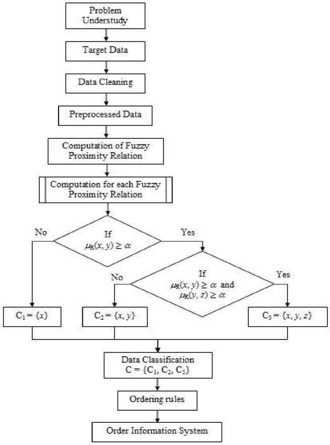
Fig. 2: Preprocessing architecture design

The fundamental step of any model is the identification of right problem. Incorporation of prior knowledge is always associated with the problem definition however; the potential validity or usefulness of an individual data element or pattern of data element may change dramatically from organization to organization because of the acquisition of knowledge and reasoning that may be involved in vagueness and incompleteness. It is very difficult for human beings to predict missing associations that is hidden in the high dimensional data. Therefore, the most important challenge is to predict data pattern and unseen associations from the accumulated high dimensional data. Hence, it is essential to deal with the incomplete and vague information in classification, data analysis, and concept formulation. To this end we use rough set on fuzzy approximation space with ordering rules in preprocess to mine suitable classification. In preprocess as shown in Fig. 1 we use rough set on fuzzy approximation spaces with ordering rules for processing data, and data classification after removal of noise and missing data. Based on the classification obtained in preprocess, we use Bayesian classification to predict decision for missing or unseen associations.

5.1 Preprocessing Architecture Design

In this section, we present our preprocess architecture design that consists of problem undergone, target data, data cleaning, fuzzy proximity relation, data classification, and ordering rules as shown in Fig. 2. Problem definition and incorporation of prior knowledge are the fundamental steps of any model. Then structuring the objectives and the associated attributes a target dataset is created on which data mining is to be performed. Before further analysis a sequence of data cleaning tasks such as removing noise, consistency check, and data completeness is done to ensure that the data are as accurate as possible. Finally for each attribute, we compute the a -equivalence classes based on the almost indiscernibility relation as discussed in section 2. The fuzzy proximity relation identifies the almost indiscernibility among the objects. This result induces the a -equivalence classes. We obtain categorical classes on imposing order relation on this classification.

• VI.    An Empirical Study on Marketing Strategies

In this section, we demonstrate the proposed model by considering a real life problem for extracting information. We consider the case study in which we study the different cosmetic company's business strategies in a country. In Table 2 given below, we consider a few parameters for business strategies to get maximum sales; their possible range of values and a fuzzy proximity relation which characterizes the relationship between parameters. We define a fuzzy proximity relation R(x , x ) in order to identify the almost indiscernibility among the objects x and x , where

R ( X i , X j ) = 1 -

I V¹' - V.\ 2( V + V )

The membership function has been adjusted in such a manner that their values should lie in [0, 1] and these functions must also be symmetric. The requirement in the numerator necessitates a major of 2 in the denominator. The companies having high expenditure in marketing, advertisement, distribution, miscellaneous, and research and development is the ideal case. But such a blend of cases is rare in practice. So, a company may not excel in all the parameters in order to get maximum sales. However, out of these parameters, some parameters may have greater influence on others. But, the attribute values on these parameters obtained are almost indiscernible and hence can be classified by using rough set on fuzzy approximation space [9] and ordering rules.

The membership function has been adjusted such that its value should lie in [0, 1] and also the function must be symmetric. The companies are judged by the sales output that is produced. The amount of sales is judged by the different parameters of the companies. These parameters form the attribute set for our analysis. Here the marketing expenditure means, all expenditure incurred for corporate promotion, which includes event marketing, sales promotion, direct marketing etc. which comes to around 6%. The advertising expenditure includes promotional activities using various medium like television, newspaper, internet etc. which comes around 36%. The miscellaneous expenditure is mainly incurred through activities like corporate social responsibility and it leads to maximum of 28%. The distribution cost includes expense on logistic, supply chain etc. and it comes around 24%. The investment made on new product development and other research activities are taken on research and development activities and it takes around 6% and the last one, the sales which basically deals with the sales that a company can produce after investing the expenditure in different fields mentioned above. The company can observe the profit by subtracting the value of the total expenditure from the value of the total sales. The data collected is considered to be the representative figure and tabulated below in Table 2.

Table 2:   Notation representation table

Parameter	Attribute	Possible range	Membership Function
Expenditure on marketing	Mkt.	[1 – 150]	1 V - V x- 1 2( V + V p
Expenditure on advertisement	Advt.	[1 – 900]	| V - V x, | 2(^ + V P
Expenditure on distribution	Dist.	[1 – 600]	। V x — V x- । 2(^ + V .)
Expenditure on miscellaneous	Misc.	[1 – 700]	| V x — V x, | 2( V + V ) xixj
Expenditure on research and development	R&D	[1 – 150]	। Vx- — Vx- । 2( V , + V )
Sales	Sales	[1– 12000]	| V x — V x, | 2( V + V, ) xixj

In the Table 3 we present the data obtained from ten different companies. However, we keep their identity confidential due to various official reasons. Here we use the notation xt , i = 1,2,3, ---ДО for different companies for the purpose of our study to demonstrate the proposed prediction model. It is to be noted that, in the information table all non-ratio figures shown in the Table 3 are ten million INR.

Table 3:   Sample information system

Comp.	Mkt.	Advt.	Dist.	Misc.	R&D	Sales
x 1	18.276	162.236	30.236	72.146	9.156	1220.586
x	2.076	5.393	6.793	8.290	0.383	215.767
x 3	0.496	1.330	0.433	2.733	0.393	42.593
x 4	0.940	0.060	0.666	5.890	1.243	166.41
x 5	27.333	38.660	16.496	24.343	1.523	561.697
x 6	7.033	866.916	508.676	637.530	38.963	11449.56
x 7	4.323	4.173	1.753	3.176	0.003	60.89
x 8	38.516	40.046	3.126	8.026	0.056	303.57
x 9	0.466	0.460	0.993	3.803	0.053	62.836
x 10	0.603	0.036	0.393	0.613	0.016	20.523

• 6.1    Preprocess of Empirical Study

Table 4:   Fuzzy proximity relation for attribute mkt.

Rx		X,	Л	x4	Л	Xs	x.	Л	Xs	xio
Л	1.000	0.602	0.526	0.549	0.901	0.778	0.691	0.822	0.525	0.532
^	0.602	1.000	0.693	0.812	0.571	0.728	0.824	0.551	0.683	0.725
Л	0.526	0.693	1.000	0.845	0.518	0.566	0.603	0.513	0.984	0.951
x4	0.549	0.812	0.845	1.000	0.533	0.618	0.679	0.524	0.831	0.891
X?	0.901	0.571	0.518	0.533	1.000	0.705	0.637	0.915	0.517	0.522
	0.778	0.728	0.566	0.618	0.705	1.000	0.881	0.654	0.562	0.579
	0.691	0.824	0.603	0.679	0.637	0.881	1.000	0.601	0.597	0.622
	0.822	0.551	0.513	0.524	0.915	0.654	0.601	1.000	0.512	0.515
	0.525	0.683	0.984	0.831	0.517	0.562	0.597	0.512	1.000	0.936
Ло	0.532	0.725	0.951	0.891	0.522	0.579	0.622	0.515	0.936	1.000

Table 5:   Fuzzy proximity relation for attribute advt.

^2	Л	X,	Л	x4			Xr	Л	Л	xio
xL	1.000	0.532	0.508	0.500	0.692	0.658	0.525	0.698	0.503	0.500
X2	0.532	1.000	0.698	0.511	0.622	0.506	0.936	0.619	0.579	0.507
	0.508	0.698	1.000	0.543	0.533	0.502	0.742	0.532	0.757	0.526
x4	0.500	0.511	0.543	1.000	0.502	0.500	0.514	0.501	0.615	0.875
*	0.692	0.622	0.533	0.502	1.000	0.543	0.597	0.991	0.512	0.501
Л	0.658	0.506	0.502	0.500	0.543	1.000	0.505	0.544	0.501	0.500
Л	0.525	0.936	0.742	0.514	0.597	0.505	1.000	0.594	0.599	0.509
^	0.698	0.619	0.532	0.501	0.991	0.544	0.594	1.000	0.511	0.501
Xs	0.503	0.579	0.757	0.615	0.512	0.501	0.599	0.511	1.000	0.573
X10	0.500	0.507	0.526	0.875	0.501	0.500	0.509	0.501	0.573	1.000

Table 6:   Fuzzy proximity relation for attribute dist.

	Л	Xj	Л	x4				Л	Л	-4o
	1.000	0.683	0.514	0.522	0.853	0.556	0.555	0.594	0.532	0.513
Xs	0.683	1.000	0.560	0.589	0.792	0.513	0.705	0.815	0.628	0.555
Л	0.514	0.560	1.000	0.894	0.526	0.501	0.698	0.622	0.804	0.976
Л,	0.522	0.589	0.894	1.000	0.539	0.501	0.775	0.676	0.901	0.871
	0.853	0.792	0.526	0.539	1.000	0.531	0.596	0.660	0.557	0.523
	0.556	0.513	0.501	0.501	0.531	1.000	0.503	0.506	0.502	0.501
	0.555	0.705	0.698	0.775	0.596	0.503	1.000	0.859	0.862	0.683
	0.594	0.815	0.622	0.676	0.660	0.506	0.859	1.000	0.741	0.612
^	0.532	0.628	0.804	0.901	0.557	0.502	0.862	0.741	1.000	0.784
Ло	0.513	0.555	0.976	0.871	0.523	0.501	0.683	0.612	0.784	1.000

Table 7:  Fuzzy proximity relation for attribute misc.

		X,		x4	-X		Xt		:4	^0
	1.000	0.603	0.536	0.575	0.752	0.602	0.542	0.600	0.550	0.508
	0.603	1.000	0.748	0.915	0.754	0.513	0.777	0.992	0.814	0.569
	0.536	0.748	1.000	0.817	0.601	0.504	0.963	0.754	0.918	0.683
Л4	0.575	0.915	0.817	1.000	0.695	0.509	0.850	0.923	0.892	0.594
	0.752	0.754	0.601	0.695	1.000	0.537	0.615	0.748	0.635	0.525
	0.602	0.513	0.504	0.509	0.537	1.000	0.505	0.512	0.506	0.501
	0.542	0.777	0.963	0.850	0.615	0.505	1.000	0.784	0.955	0.662
	0.600	0.992	0.754	0.923	0.748	0.512	0.784	1.000	0.821	0.571
	0.550	0.814	0.918	0.892	0.635	0.506	0.955	0.821	1.000	0.639
-Чо	0.508	0.569	0.683	0.594	0.525	0.501	0.662	0.571	0.639	1.000

R3			Xg	A	x=		X-		S	^10
Xl	1.000	0.540	0.541	0.620	0.643	0.690	0.500	0.506	0.506	0.502
	0.540	1.000	0.994	0.736	0.701	0.510	0.508	0.628	0.622	0.540
	0.541	0.994	1.000	0.740	0.705	0.510	0.508	0.625	0.619	0.539
x4	0.620	0.736	0.740	1.000	0.949	0.531	0.502	0.543	0.541	0.513
	0.643	0.701	0.705	0.949	1.000	0.538	0.502	0.535	0.534	0.510
	0.690	0.510	0.510	0.531	0.538	1.000	0.500	0.501	0.501	0.500
	0.500	0.508	0.508	0.502	0.502	0.500	1.000	0.551	0.554	0.658
	0.506	0.628	0.625	0.543	0.535	0.501	0.551	1.000	0.986	0.722
	0.506	0.622	0.619	0.541	0.534	0.501	0.554	0.986	1.000	0.732
-Чо	0.502	0.540	0.539	0.513	0.510	0.500	0.658	0.722	0.732	1.000

Table 9:   Fuzzy proximity relation for attribute sales.

R5			Xg	x4			X-		Xg	^10
X1	1.000	0.650	0.533	0.619	0.815	0.596	0.547	0.699	0.548	0.516
	0.650	1.000	0.644	0.995	0.777	0.518	0.720	0.915	0.725	0.586
	0.533	0.644	1.000	0.703	0.570	0.503	0.911	0.623	0.903	0.825
x4	0.619	0.995	0.703	1.000	0.728	0.514	0.767	0.854	0.774	0.609
	0.815	0.777	0.570	0.728	1.000	0.546	0.597	0.850	0.600	0.535
	0.596	0.518	0.503	0.514	0.546	1.000	0.505	0.525	0.505	0.501
	0.547	0.720	0.911	0.767	0.597	0.505	1.000	0.667	0.992	0.752
	0.699	0.915	0.623	0.854	0.850	0.525	0.667	1.000	0.671	0.563
	0.548	0.725	0.903	0.774	0.600	0.505	0.992	0.671	1.000	0.746
	0.516	0.586	0.825	0.609	0.535	0.501	0.752	0.563	0.746	1.000

Now on considering the almost similarity of 85% i.e. , a >  0.85 it is observed from Table 4 that R_x ( x , x ) = 1; R ( x , x ₅) = 0.901 ; R ( x ₂, x ₂) = 1 ; R ( x ₃, x ₃) = 1 ; R 1 ( X 3 , X 9 ) = 0.984; R 1 ( x 3 , x _w) — 0.951; R 1 ( x ₄, x ₄) — 1; R 1 (x 4 , x _w) = 0.891; R 1 (X 5 , X 5 ) — 1; R 1 ( x ₅, x 8 ) = 0.915 ; R ( x ₆, x ₆) = 1; R ( x ₆, x ₇) = 0.881. Thus, the companies x , x ₅, x₈ are a -identical. Similarly, x ₆, x₇ are a -identical; x ₃, x ₄, x ₉, x₀ are a -identical and x ₂ is a -identical. Therefore, we get

U I R 1  ^— { ^{{ x} 1 , ^x 5 , ^x 8^} , ^{{ x} 6 , ^x 7^} , { ^x 3 , ^x 4 , ^x 9 , ^x 10 ^} , { x 2 ^{} }}

Therefore, the values of the attribute expenditure on marketing are classified into four categories namely very low, low, average and high and hence can be ordered.

U! R2 — {{x1 }, {x2 , x7}, {x3 }, {x4 , x10 }, {x5 , x8}, {x6 }, {x9 }} uiRa

U/R 4 ^a

= {{ x i , x 5 },{ x ₂},{ x ₃, x 4 , x ₇, x 8 , x 9 , x ₁₀},{ x ₆}}

^{— {{ x} 1 ^} , ^{ x 2 , ^x 3 , x 4 , ^x 7 , ^x 8 , ^x 9^} , ^{ x 5 ^} , ^{ x 6 ^} , ^{{ x} 10 ^}}

^U/ R 5    ^{{{ x} 1 ^} , ^{ x 2 , ^x 3^} , ^{ x 4 , ^x 5^} , ^{ x 6 ^} , ^{ x 7 ^} , ^{{ x} 8 , ^x 9^} , ^{{ x} 10 ^}}

^U/^R 6 ^{— { { x} 1 ^} , ^{ x 2 , x 4 , ^x 5 , ^x 8^} , ^{{ x} 3 , ^x 7 , ^x 9^} , ^{{ x} 10 ^} , ^{ x 6 ^}}

From the above classification, it is clear that the values of the attribute expenditure on advertisement are classified into seven categories namely poor, very low, low, average, high, very high and outstanding. The values of the attribute expenditure on distribution are classified into four categories namely low, average, high, and very high. The values of the attribute expenditure on miscellaneous are classified into five categories namely very low, low, average, high and very high. The values of the attribute expenditure on research and development are classified into seven categories namely poor, very low, low, average, high, very high and outstanding. Finally, the values of the attribute sales are classified into five categories namely very low, low, average, high and very high. Therefore the ordered information system of the business strategies of different cosmetic companies of Table 3 is given below in Table 10.

Table 10: Order information system

Comp.	Mkt.	Advt.	Dist.	Misc.	R&D	Sales
x 1	High	Very high	High	High	Very high	High
x 2	Low	Avg.	Avg.	Low	Avg.	Avg.
x 3	Very low	Low	Low	Low	Avg.	Low
x 4	Very low	Poor	Low	Low	High	Avg.
x 5	High	High	High	Avg.	High	Avg.
x 6	Avg.	Outstanding	Very high	Very high	Outstanding	Very high
x 7	Avg.	Avg.	Low	Low	Poor	Low
x 8	High	High	Low	Low	Low	Avg.
x 9	Very low	Very low	Low	Low	Low	Low
x 10	Very low	Poor	Low	Very low	Very low	Very low

: High Average Low Very Low

: Outstanding Very High High Average Low Very Low Poor

: Very High  High  Average  Low

: Very High  High  Average  Low Very Low

: Outstanding Very High High Average Low Very Low Poor

: Very High High Average Low Very Low

• 6.2    Postprocess of Empirical Study

Bayesian classification analysis can do the data classification. However data are already classified in preprocess. The objective of this process is to use Bayesian classification to predict the unseen association rule from the order information system and hence to get better knowledge affecting the decision making. In order to show post processing analysis, we consider an unseen association of attribute values T = {Mkt. = High, Advt. = Average, Dist. = Low, Misc. = Average, R&D = High} to predict the decision ‘sales’. Let us take T ^— {t¹, t ², t ³, t ⁴, t 5^} , where t ¹ is Mkt. = High; t ²

is Advt. = Average; t ³ is Dist. = Low; t ⁴ is Misc. =

Average; and t ⁵ is R&D = High. From the preprocessing, it is clear that the decision ‘sales’ has 5

P ( 1 5 I C 1 ) =

and

C          CC classes say 1 = Very high, 2 = High, 3 =Average,

C, = Low      , C, = Very . _D    P ( 1 | C ) = 0 _f

⁴         , and ⁵          low. But, ^{i 1}      for

P ( C 1 ) =

i = 1,2,3,4,5

...  p(C) = 1/10          4         + with     1        . Thus, it dominates

the classification of future instances as Bayes classifier

P ( t | C )

multiplies ^{i 1} together. Therefore, by using m- estimate we get:

p ( t i | C 1 ) =

0 + 4Q)

1 + 4

P ( 1 2 C 1 ) =

0 + 7( 7 )

1 + 7

P ( 1 3 I C 1 ) =

0 + 4( 4 )

1 + 4

P ( 1 4 I C 1 ) =

0 + 5( 5 ) 1 + 5

0 + 7( 7 ) 1 + 7

1 + 5( 5 )

10 + 5

Therefore, by using Bayesian classification we get

P ( C 1\ T ) = П P ( t i I C 1 ) P ( C 1 )

i = 1

= 1 x 1 x 1 x 1 x 1 x £ = 0.0000138

5    8    5    6    8    15

Similarly, we get

P ( C ₂ I T ) = 0.0000277; P ( C | T ) =

0.000516;   P ( C ₄| T ) = 0.0000544;  _and   P ( C ₅| T ) =

0.0000173 . From the above computations it is clear

P ( C | T )

that     3     is maximum. Therefore, it is clear that the above unseen association of attribute values belongs C = to the decision class 3 Average. Keeping view to the length of the paper, some of the unseen association of attribute values and its corresponding decision are presented in Table 11.

Table 11: Prediction of unseen associations

Unseen associations	Mkt.	Advt.	Dist.	Misc.	R&D	Sales
1	Very low	High	Low	Low	High	Avg.
2	Very low	Avg.	Low	Low	Avg.	Low
3	Very low	High	Low	Low	Avg.	Avg.
4	High	Very high	Very high	High	Outstanding	High
5	High	Avg.	Low	Low	Avg.	Avg.
6	High	High	Low	Low	High	Avg.
7	Very low	Avg.	Low	Low	Low	Low
8	Very low	Avg.	Low	Low	High	Avg.
9	Avg.	Avg.	Low	Low	Low	Low
10	High	Poor	Low	Low	High	Avg.
11	Avg.	Avg.	Low	Low	Avg.	Low

VII.Conclusion

Prediction of unseen or missing associations of attribute values is a challenging task in the study of high dimensional database. In general, Bayesian classification is used to predict the unseen association rule. However, it is not directly applicable in case of information system containing almost indiscernible attribute values. In order to overcome this problem the proposed prediction model uses both rough computing with ordering rules and Bayesian classification. The model identifies the almost indiscernibility between the attribute values in the preprocess phase whereas

Bayesian classification is used in the post process to predict the decision. This helps the decision maker a priori prediction of sales. We have taken a real life example of 10 cosmetic company’s database according to different attributes and shown how analysis can be performed by considering the proposed model. We believe that, rough computing with ordering rules together with Bayesian classification can be used to find furthermore information regardless of the type of associations based soft computing. We also believe that the proposed model is a useful method for decision makers and mining knowledge.