Prediction of performance point of semi-rigid steel frames using artificial neural networks

Published Online October 2019 in MECS

• I.    Introduction

  Past destructive earthquakes (e.g. 1989 Loma Prieta; 1990 Manjil-Rudbar; 1994 Northridge) have left their signature below the documents of the economical and life losses reported then. In accordance with the seismic design codes, some degree of damage is expected for ordinary buildings subjected to design basis earthquakes. Although preventing the natural earthquake occurrence is beyond the human control, the ways of mitigating such losses have been the enforced interest of researchers and engineering communities. The inappropriate performance of structures under the past destructive earthquakes caused the communities to eliminate the unexpected losses then. One of the modern methodologies gaining significant attention is the performance-based seismic design (PBSD) [1]. Over the last 30 years, the conceptual framework of PBSD was developed by the various guidelines published by the well-known engineering associations such as Structural Engineers Association of California [2], Applied Technology Council [3], and Federal Emergency Manage Agency [4].

Conceptually, it is expected to have different seismic performance levels of structures due to various structural seismic behaviors and hazard levels. Because of this, the abovementioned guidelines have introduced different seismic performance levels (or objectives) corresponding to the different hazard levels and thus, each structure of interest should be evaluated based on its relevant performances and hazard levels. Based on the studies so far carried out, it was found that the steel frame structures experience some degree of nonlinearity under severe earthquakes and thus, the single parameters of strength could not be accepted for the seismic analysis and design. Hence, as the guidelines have recommended, the analysis and design process can be carried out using the expected seismic performance (e.g. force and/or deformation) of the subject structure. In fact, in order to design or retrofit the new and existing buildings respectively, a performance objective is chosen by owner/designer based on the defined performance and hazard levels in the mentioned guidelines [4].

Performance-based seismic analysis and design of structures requires determining the performance point. The performance point is obtained from the intersection point of target displacement and base shear on the pushover curve of the subject structure. To determine the performance point, nonlinear static analysis is required to be performed. The process is case-sensitive and the nonlinear analysis is inherently a time-consuming process which needs high computational efforts. An alternative way is to predict the point using soft computing-based predictive tools. Over the last three decades, the much computational burden of computational approaches and sometimes their weakness were resulted in discovering the soft computing-based approach, which have been increasingly applying in the different aspects of complex engineering problems. Soft computing-based approach includes several tools such as evolutionary algorithms, artificial neural networks (ANNs), support vector machine (SVM), and fuzzy logic. These predictive tools are typically used for modeling the nonlinear dependency of input parameters to output value(s) where the conventional approaches fail or perform poorly [5].

In the recent decades, soft computing-based approach have been widely using to simplify the complex problems in a broad range of civil engineering problems (e.g. [518]). Some of the relevant studies to application of ANNs in structural engineering problems are described herein. Adeli and Karim [19] used ANN model for design optimization of cold-formed steel beams. A wavelet neural network was used by Salajegheh and Heidari [15] to optimal seismic design of structures. The successful applications of a radial basis function (RBF), selforganizing RBF, and fuzzy self-organizing RBF, and fuzzy wavelet RBF neural networks in predicting the elastic time-history responses required for optimal seismic design of steel structures were reported by Salajegheh and his colleagues [13, 14, 20]. Three different ANNs including feed-forward Levenberg-Marquardt backpropagation (BP) neural network, a recurrent neural network, and a RBF neural network were used by Pannakkat and Adeli [21] to predict the magnitude of the largest seismic event in the following month based on the analysis of eight mathematically computed parameters known as seismicity indicators. Seyedpour et al. [16] conducted a research on optimal shape design of arch dams under earthquake loads. To reduce the computational burden of the optimization procedure, they approximated the dam seismic responses using wavelet neural networks and fuzzy inference system. Naderpour et al. [22] used a BP neural network to estimate the compressive strength of FRP-confined concrete specimens using a large number of experimental data. Alavi and Gandomi [23] formulated three principal ground motion parameters of peak ground acceleration, peak ground velocity and peak ground displacement by using a hybrid ANN coupled with simulating annealing. Lagaros and Papadrakakis [24] used ANNs to accurately prediction of inelastic dynamic responses of 3D framed buildings subjected to three earthquake levels. Ahmadi et al. [11] employed a BP neural network to estimate the capacity of concrete filled steel tube short columns subject to short term axial loads. A new neural network as wavelet cascade-forward BP was also employed for reducing computational burden of performance based optimal seismic design of steel frame structures [25]. In fact, the mentioned network was used to accurately prediction of inter-storey drift ratio based on pushover analysis. Gandomi and Roke [5] assessed the performance of a hybrid ANN and genetic programming in predicting the punching shear strength of concrete slabs by using the experimental data. Gholizadeh and Mohammadi [12] used a wavelet BP to predict the inelastic responses needed for reliability-based seismic optimization of steel frames. Heidari et al. [26] used a BP neural network to predict the compressive strength of waste concrete. Recently, Kotsovou et al. [27] reported a comprehensive study on the failure assessment of reinforced concrete exterior beam-column joints using ANNs that the results were compared to the analytical methods indicating the accuracy of prediction model. More recently, Gharehbaghi et al. [6] used ANN and SVM methods to estimate the inelastic seismic responses of reinforced concrete structures.

The aim of this paper is to predict the performance point of steel frame structures with semi-rigid connections, known as semi-rigid steel frames (SRSFs), by using ANNs. Several SRSFs were modeled and pushover analyses were carried out to derive the capacity curve. Ten input variables including number of stories, number of bays, bays width, cross sectional moment of inertia of beams, cross sectional area of columns, cross sectional area of braces, design basis acceleration, soil type, rigidity degree of connections and existence or nonexistence of soft story were considered in the prediction. The actual results were obtained at the presence of different earthquake intensity levels and soil types. The model prediction has two output values of roof displacement and base shear requiring for determining the performance point. Eleven BP neural networks and an RBF neural network were used for the prediction and the results are compared together herein.

• II.    Steel Frames with Semi-Rigid Connections

The behavior of beam-column connection has significant effects on the both elastic and inelastic global behavior of steel frame structures. In order to capture the realistic behavior of the connection, its properties need to be modelled accurately. Although the beam-column connections are assumed as pinned and/or fixed in practical designing, experimental and analytical studies have shown that they do not behave as pinned and/or fixed and the actual behavior lies somewhere between these two idealized models. Moreover, studies have shown that there is a nonlinear dependency between the applied moment and the rotation of beam-column connection. A typical moment-rotation relationship is shown in Fig. 1.

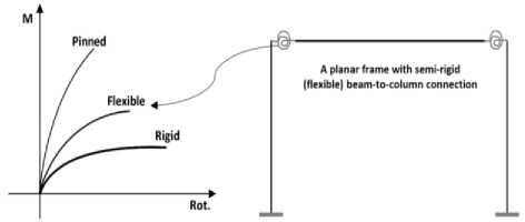
Fig.1. A typical moment-rotation (M-Rot.) relationship of steel beamcolumn connections.

There are a large number of works dealt with the experimental and numerical seismic assessment of SRSFs. Some of the works are investigated herein. Static and cyclic performance of semi-rigid steel beam-column connections was investigated by Azizinamini and Radziminski [28]. They found that the beam section to which the connection elements are framed, the thickness of the flange angles, and the gage in the leg of the flange angle attached to the column are the most influential geometric parameters on the static moment-rotation behavior of the connection. Nader and Astaneh-asl [29] compared the dynamic behavior of semi-rigid and rigid steel moment frames. They also conducted a study on the dynamic behavior of flexible, semi rigid and rigid steel frames by using a shake table test. Elnashai et al. [30] investigated the cyclic and seismic response of SRSFs. They studied the effect of connection stiffness on the overall stiffness of the frame, inter-story drift criteria and overstrength factor. Awkar and Lui [31] evaluated the seismic response of multi-storey SRSFs. It was shown that although the connection flexibility tends to increase the inter-story drift at upper stories, it reduces the base shear and overturning moments of the frames. It was also concluded that connection flexibility will result in the frame periods to spread over a wider spectrum which increases the contributions of higher modes in structural responses. The nonlinear P-Delta effects on the response of SRSFs was investigated by Valipour and Bradford [32]. Nguyen and Kim [33] presented a numerical procedure to assess the three dimensional SRSFs using nonlinear timehistory analysis method. The effects of material, geometry and connection nonlinearities were considered in their presented procedure. Razavi and Abolmaali [34] investigated the seismic performance of a 20-story hybrid steel frame with several different patterns and locations of semi-rigid connections. They found more collapse margine ratio for hybrid frames compared with a conventional frame having rigid connections. Yu and Zhu

• [35]    evaluated the nonlinear dynamic collapse of SRSFs using finite particle method. They found that the flexibility of connections which increases the energy dissipation capacity due to hysteretic damping, could overestimate the overall stiffness and loading capacity of the frames, avoiding the frames to resonate under seismic load with a dominant frequency close to the natural frequency of the frames compared with those of with rigid connections. Faridmehr et al. [36] investigated the seismic performance of steel frames with semi-rigid connections. They showed that the more flexibility of semi-rigid connection causes more decreasing in base shear demand during earthquake. Pirmoz and Liu [37] presented a direct displacement-based design method to seismic design of SRSFs. Some of researchers have dealt with the optimization of SRSFs. For example, Kameshki and Saka [38] presented a work on optimization of SRSFs. They used Frye–Morris polynomial model for semi-rigid connections. Oskouei et al. [39] presented a framework for optimization of seismic behavior of SRSFs using genetic algorithm. Both linear and nonlinear analyses were used in the process. Yassami and Ashtari [40] presented the optimal design of SRSFs. They concluded that the SRSFs may result in 30% increase in the roof displacement compared with the frames with rigid beamcolumn connections. Also, it was revealed that about 1020 % decreasing in structural weight of frames with semirigid connections compared with those of rigid connections is expected.

• III.    Nonlinear Static Procedure

One of the most preferred structural analysis methods for performance-based seismic evaluation and design is nonlinear static analysis approach. In the simplified version of the approach, only the structural members including beams and columns (and braces) are modeled and the nonlinear behavior is considered as lumped or distributed plasticity. Then the subject structure is pushed until reaching a certain roof displacement and seismic evaluation is conducted based on the response of the structure.

Based on the abovementioned guidelines such as FEMA [4], the subject structure should have enough capacity to withstand a specified roof displacement for a specific earthquake. This is called as the target displacement and, for instance, for Life Safety performance level is defined as an estimate of the likely building roof displacement under the design earthquake. Because the mathematical model accounts directly for the effects of material inelastic response, the calculated internal forces will be reasonable approximations of those expected during the design earthquake. Hence, the internal forces and deformations are evaluated when the roof displacement is equal to the target displacement. Two common methodologies available to determine the target displacement are: (i) capacity spectrum method and (ii) displacement coefficient method. In this paper, the displacement coefficient method is used to obtain the target displacement. If the Nonlinear Static Procedure

(NSP) is selected for seismic analysis of the building, a mathematical model incorporating the nonlinear loaddeformation characteristics of the individual components and elements of the building should be subjected to monotonically increasing lateral loads representing inertia forces in an earthquake until a target displacement is exceeded [4].

The displacement coefficient method was firstly proposed by Nassar and Krawinkler [41] which is the recommended method by FEMA-356 guideline [4]. In this method, the linear elastic response of an equivalent single degree of freedom (SDOF) system is modified by multiplying it by a series of coefficients to estimate the target displacement of the structure of interest. In this method, the structure is pushed with a specific distribution of the lateral loads until the target displacement is reached. The target displacement can be calculated as follow [4]:

T ²

§ t = C 0 CC 2 C 3 S a ^1 g (1) к 2 П )

where C ₀ is the modification factor to relate spectral displacement of an equivalent SDOF system to the roof displacement of the subject building; C ₁ is the modification factor to relate expected maximum inelastic displacements to displacements calculated for linear elastic response; C 2 is the modification factor to represent the effect of pinched hysteretic shape, stiffness degradation and strength deterioration on maximum displacement response; C 3 is the modification factor to represent increased displacements due to dynamic P-∆ effects; S _a is the response spectrum acceleration at the effective fundamental period and damping ratio of the building in the direction under consideration; g is the gravity constant; and T _e is the effective fundamental period in the direction under consideration which shall be determined based on the idealized force-displacement curve defined in FEMA-356 [4].

• IV.    ANN Technique

Artificial neurons and a simple model of a biological neuron are the main body parts of an ANN which is arranged on a set of layers. ANNs have distinct features in learning the experiences and examples, and matching with changing position. Engineers often deal with the big and/or incomplete data where the ANNs have been highly recommended to have the applications such as function approximation, time series prediction, classification, recognition and system control. Thanks to their high capability and simplicity in using the mentioned applications, ANNs have received great attention among researchers (e.g. [5-7, 16, 17, 20, 24, 26, 42-51]). In this paper, two well-known and most used neural networks of BP and RBF were used for the prediction. A brief description of both BP and RBF is expressed herein.

• A.    Back Propagation (BP) ANNs

The BP method was firstly presented by Rumelhart et al. [52]. The ANN trained by BP method is called as BP ANN. BP was created by generalizing the Widrow-Hoff learning rule to multiple layer networks and nonlinear differentiable transfer functions. Input vectors and the corresponding target vectors are used for training a network until it can approximate a function. BP commonly uses a gradient descent algorithm, as the Widrow-Hoff learning rule, in which the network weights are moved along the negative of gradient of the performance function.

BP is usually used as a part of algorithms that optimize the performance of the network by adjusting the weights, for example, in the gradient descent algorithm. The overall procedure of the gradient computation and its use in the optimization using basic calculus independent of the optimization algorithm is simple. After choosing an appropriate structure for the ANN and assuming initial values for their weights, the optimization algorithm repeats two phase cycles of propagation and weight optimization. In the propagation phase, the presented input vector to the network is propagated through the network, layer by layer, until reaching the output layer. In fact, in lieu of an input vector, an output is obtained. The network output is compared with a desired output and the error is calculated for each of the neurons in the output layer. The errors derivation with respect to network weights is calculated then. In the second phase, this gradient is fed to the optimization method in order to update the weights. The procedure is repeated to minimize the errors until reaching an acceptable error. The computations are sequentially carried out within the series layers and the final output vector is obtained as predicted values.

• B.    Radial Basis Function (RBF) Neural Networks

An ANN that uses RBF as its activation function is so-called as RBF ANN. The output of the network is a linear combination of RBFs of the inputs and neuron parameters. RBFs were firstly used for designing the neural networks by Broomhead and Lowe [53]. Because of their fast training, simplicity and performance generality, RBF neural networks have been widely using in the field of civil and structural engineering (e.g. [13, 14, 43]). It has been shown that RBF ANNs are universal predictors and can predict any continuous function with arbitrary precision [54, 55]. These networks are feed forward of networks of two layers. In order to train the hidden layer of RBF networks, no training is accomplished and the transpose of the training input matrix is taken as the layer weight matrix. Also, a supervised training algorithm is employed to adjust output layer weights [56].

• V.    Prediction Methodology

As mentioned, this paper aimed at predicting the performance point of SRSFs. The performance point is the value of target displacement (called as TD herein) corresponding to a demand base shear (called as BS herein). Hence, these two parameters of BS and TD were considered as two output values to be predicted using ANNs. For this purpose, several SRSFs (our samples herein) were modeled and pushover analysis of the models was carried out. Then, the subject output values were calculated. Ten input variables including number of stories, number of bays, bays width, cross sectional moment of inertia of beams, cross sectional area of columns, cross sectional area of braces, design basis acceleration, soil type, rigidity degree of connections and soft story (existence or nonexistence) were considered in the prediction. The variables are shown in the Fig. 2.

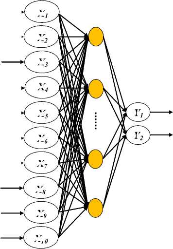
The number of input-output neurons is determined largely based on the requirements, but there is no rule for determining the number of neurons in the hidden layer. Therefore, it is assumed that all the trained networks have a structure with 10 neurons in input layer and two neurons in output layer. Since, there is no rule to obtain the suitable number of neurons in the hidden layer directly, with changing the number of hidden layer from 4 to 20, the best number of neurons was obtained using a trial-and-error process. The fewer periods and less time required to achieve less error in testing and training of the ANNs were the criterion used to determine the best number of neurons in hidden layer. The sigmoid and hyperbolic tangent transfer functions were used in BP ANNs. Fig. 3 shows the variation of these functions along variable x.

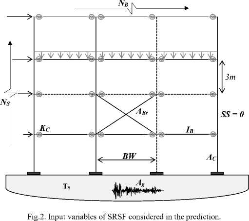
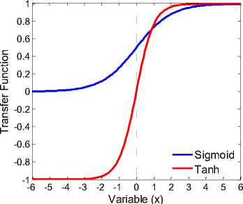
Fig.3. Variation of transfer functions (Sigmoid and Tanh) used for variable x.

• VI.    Worked Examples

• A.    Modeling and Assumptions

  Thirty-five steel moment frames were designed using SAP2000 [57] software. The number of bays was

considered to be 1 to 5, and the number of stories was considered in the range of 2 to 8 stories, both with incremental step of 1. The length of each bay was considered between 3m and 5m (by assuming an increasing step of 1m) and the height of each story was considered to be equal to 3m.

Steel sections of IPE and IPB were respectively used for beam and column cross sections. Double channel (UNP) section was also used for the braces. The dead load was assumed equal to 500 kg/m2 for all the floors; and live loads were assumed equal to 200 and 150 kg/m2 respectively for the roof and rest floors. The equivalent static loading was applied based on Iranian seismic design standard (No. 2800) [58]. It was assumed that the structures are constructed in a zone with high seismicity and on a site with soil type II, and have important factor of 1.0. The connection of columns at the base was considered as rigid. After design step, the beam-column connections of the designed frames were modified and modeled as semi-rigid. For this purpose, the stiffness of the connections was modified to have almost 20 to 90% (considering 18 ratios in this range) with respect to the initially designed frames. The variations mentioned and the stiffness modifications were resulted in 427 SRSFs. The beams, columns and braces were modeled such that they are capable of considering material nonlinear behavior. The P-А effect was considered in the modeling and analyses. After modeling the frames and by applying pushover analysis, the capacity curve of the frames was obtained. The target displacement of the frames, considering three hazard levels of moderate, high and very high seismicity for three soil classes, were determined corresponding to the LS performance level. For this purpose, the displacement coefficient method available in FEMA-356 [4] was used. The mentioned classification was resulted in 3057 samples.

While the soil type assumed for initial design was type II, to have a wide range of samples, three soil types were considered in generating samples. In Iranian seismic design standard (No. 2800) [58], the differences among soil types can be identified using the parameter of T _s which is equal to 0.4s, 0.5s and 0.7s for soil types of I to

III, respectively. The design basis acceleration was also varied from 0.25g to 0.35g which is corresponding to the relatively low to high intensity of seismicity levels (based on seismic risk analysis in Iran). The effect of soft story was also considered in the results. To achieve this, a braced system was modeled in one of the bays of the subject frame in all the stories. When a story is not braced, it means that the story is susceptible to experience soft story. The range of all the variables used in this study are listed in Table 1. The parameters (inputs) used in this study are named as: (a) N S : number of stories; (b) N B : number of bays; (c) BW : bay width; (d) I B : moment of inertia of beam section; (e) A C : cross section area of column; (f) A _Br : cross section area of column; (g) K _C : relative rotational stiffness of beam-column connection; (h) T _s : a period introducing the soil type; (i) A _g : design basis acceleration; (j) SS : introducing soft story formation (0 for soft story).

Table 1. The minimum and maximum of input variables used.

Limits	Inputs
	N S	N B	BW (cm)	I B (cm4)	A C (cm2)	A Br (cm2)	K C	T S	A g	SS
Min.	2	1	300	1317	65.3	11.17	0.2	0.4	0.25	0
Max.	8	5	500	8356	149	34	0.9	0.7	0.35	1

• B.    ANNs Architecture Used

  In this study, feed forward BP and RBF ANNs with three layers were used. The architecture of the network is shown in Fig. 4. To complete the design of the ANNs, the number of neurons was changed from 4 to 20, and then a trail-and-error process was performed to find the most appropriate number of neurons. Two transfer functions of sigmoid and hyperbolic tangent were used in the hidden layer. In this research, 3057 samples were used which among them, 1835 samples (60% of all samples) were used for training the network and the residual samples (1222) were considered for testing process. Before applying the samples, the input variables were normalized to be located between 0.0 and 1.0 as follows:

x - x -

* x =------min-                    (2)

x - x -max     min where sx is the normalized value, xmin and xmax are the lower and upper bonds of x variable.

The mean square error ( MSE ) measurement of 0.01% was used to stop the training process. The maximum number of iteration equal to 5000 was considered as a second criteria for stopping the ANN training process. Also, the tolerance of two sequence iterations was used as 10^-10 as third criteria. Three statistic error measurements of mean square error ( MSE ), mean absolute error ( MAE ) and square of correlation coefficient ( R² ) were used to validate the training ANN and testing its performance. The mentioned error measurements are computed as follows:

n ²

MSE = - £( у,- t^ n i = l

N B

I B

ABr

A C

N S

K C

T S

BW

SS

A g

X 1

X 2

X 3

Y 1

X 5

Y 2

X 6

X 8

X 9

X 10

X 7

X 4

B

T

Fig.4. Topology of a feedforward ANNs used.

MAE = ^-V l y L_ n1= - t i

R =

∑ _i ⁿ _{= 1}( y _i - y _i )( t _i - t _i ) ∑ _i ⁿ _{= 1}( y i - y i )² ∑ _i ⁿ _{= 1}( t i - t i )²

where y i and t i are the predicted and actual outputs; y is average value of the predicted outputs; and n is the number of samples used. As mentioned, the actual output values were generated by SAP2000 [57]. Lower MSE and MAE show a better performance of predictive tool. In a addition, the R² values of near 1.0 indicate a best correlation between actual and predicted inputs. Note that R² is the square of R which is expressed by Eq. (5).

BP with eleven algorithms listed in Table 2 and RBF ANNs were used for the prediction. In the first step of the prediction process, 60% of data were used randomly for training and the rest were used for testing process. The same data were used for all 12 ANNs (11 BP and one RBF ANNs) introduced. The best number of neurons was found for the ANNs corresponding to the both sigmoid and hyperbolic tangent as nonlinear transfer functions. The ANN parameters which was used to the prediction process are listed in Table 3. The values listed herein were obtained based on a pre-evaluation using a trial-and-error process.

Table 2. The ANN properties used.

NO.	Algorithm abbreviation	Description
1	BP- GDM	Gradient Descent with Momentum
2	BP- GDA	Gradient Descent with Adaptive linear
3	BP- GDX	Gradient Descent with momentum and adaptive linear
4	BP- R	Resilient
5	BP- CGF	Fletcher-Powell Conjugate Gradient
6	BP- CGP	Polak-Ribiere Conjugate Gradient
7	BP- CGB	Conjugate Gradient with Powell/Beale Restarts
8	BP- SCG	Scaled Conjugate Gradient
9	BP- BFGS	BFGS Quasi- Newton
10	BP- OSS	One Step Secant
11	BP- LM	Levenberk-Mrguardt

Table 3. The ANN properties used.

ANN	Number of Training	Number of Testing	Goal	Epoch	Learning Rate	Momentum Constant	ANN structure I:N:O(a)(TF(b))
BP- GDM	1835	1222	0.0001	5000	0.9	0.5	10:10:2
BP- GDA	1835	1222	0.0001	5000	variable	-	10:6:2
BP- GDX	1835	1222	0.0001	5000	variable	0.5	10:6:2 (T(c)) 10:14:2 (S(d))
BP- R	1835	1222	0.0001	5000	-	-	10:10:2 (T) 10:8:2 (S)
BP- CGF	1835	1222	0.0001	5000	-	-	10:18:2 (T) 10:20:2 (S)
BP- CGP	1835	1222	0.0001	5000	-	-	10:8:2
BP- CGB	1835	1222	0.0001	5000	-	-	10:13:2 (T) 10:15:2 (S)
BP- SCG	1835	1222	0.0001	5000	-	-	10:17:2 (T) 10:15:2 (S)
BP- BFGS	1835	1222	0.0001	5000	-	-	10:20:2 (T) 10:17:2 (S)
BP- OSS	1835	1222	0.0001	5000	-	-	10:16:2 (T) 10:17:2 (S)
BP- LM	1835	1222	0.0001	5000	-	-	10:19:2
RBF	1835	1222	0.0001	Max. Nerons		Spread ( σ i )	10:263:2
				300		1.475

• C.    Prediction: First Try

After constructing the suitable ANNs for the defined prediction process, the performance of the networks was evaluated in both training and testing process using the statistic error measurements mentioned. In addition, running time and the number of epochs to reach the best prediction were determined which are listed in Table 4.

As can be seen in this table, there is no significant difference between the running time of prediction considering sigmoid and hyperbolic tangent (as transfer functions) with same ANN architecture. For BP-GDM, the hyperbolic tangent shows better correlation and less MAE compared with sigmoid. Because of having high MSE and MAE, the BP-GDM performance is not acceptable in general. This is same for BP-GDA. Regarding BP-GDX which uses a combination of the two former algorithms (i.e. GDM and GDA), the ANN performance is slightly improved. As shown in Table 4, although the running time of the Resilient algorithm is similar to that of for the gradient based algorithms, it has significantly improved the BP performance in terms of the errors. The running time for sigmoid transfer function is less than that of for hyperbolic tangent, but the errors are almost similar for both transfer functions used. Based on the statistic errors calculated for conjugate gradient based algorithms which were used in BP networks (including CGF, CGP, CGB and SCG), they yielded a good prediction in general. Although the run time of BP-SCG is more than other BP-ANNs with conjugate gradient based algorithms, this network with hyperbolic tangent transfer function is the most accurate one among them to predict TD and with sigmoid transfer function is the most accurate ANN to predict BS. BP-BFGS with hyperbolic tangent transfer function shows less MAE and more R2 considering about four times more running time compared with BP-SCG. In addition, the BP-OSS has a reasonable and good prediction results. Based on Table 4, the BP-LM network with hyperbolic tangent transfer function accurately predicts the TD and when it applies sigmoid function, it results in a good prediction for BS. Likewise, the errors obtained for RBF network shows its good performance.

Table 4. The train and test results for TD and BS.

ANN	TF	Epoch	Time (s)	MSE (%)		BS		TD
						MAE (%)	R2 (%)	MAE (%)	R2 (%)
				Train	Test	Test	Test	Test	Test
BP- GDM	T	5000	50.1	17.3	17.4	15.2	90.8	23.4	95.3
	S	5000	52.0	29.7	32.44	19.3	84.4	37.6	90.0
BP- GDA	T	5000	42.6	15.68	17.14	14.7	92.0	35.6	92.0
	S	5000	41.5	33.99	34.6	23.1	80.4	36.9	80.4
BP- GDX	T	5000	43.8	10.7	11.5	11.6	94.0	16.9	94.8
	S	5000	54.2	23.1	23.5	17.3	88.6	30.9	92.9
BP-Resilient	T	5000	53.9	3.35	3.66	5.7	98.2	9.2	98.9
	S	5000	43.0	5.4	6.9	5.5	98.1	9.3	98.6
BP- CGF	T	3306	99.1	2.7	3.2	4.7	98.7	11	98.7
	S	2360	80.8	3.9	4.5	5.8	97.9	10.9	98.5
BP- CGP	T	2652	56.7	3.06	3.46	5.6	98.1	9.8	99.0
	S	1510	30.4	4.9	5.35	6.3	97.6	11.1	98.1
BP- CGB	T	4349	109.3	2.07	2.5	4.7	98.6	7.5	99.3
	S	4036	112	2.28	3	4.7	98.7	10.6	98.9
BP- SCG	T	5000	118.1	0.0188	0.0256	4.7	98.5	7.0	99.4
	S	5000	114.6	0.0198	0.026	4.5	98.8	8.5	99.1
BP- BFGS	T	5000	426.2	1.09	1.81	3.8	99.0	6.3	99.5
	S	5000	320.8	1.49	2.02	4.5	98.9	7.0	99.4
BP- OSS	T	5000	126.1	3.15	3.53	5.2	98.3	11.0	98.8
	S	5000	124.6	4.08	4.92	6.8	97.7	12.6	98.4
BP- LM	T	5000	680.5	1.1	1.84	3.5	99.0	6.6	99.5
	S	5000	713.5	1.13	1.72	3.9	99.0	6.3	99.5
RBF	-	263	100.8	0.999	1.99	4.0	98.9	6.5	99.4

Table 5. The train and test results for TD and BS.

ANN	AF	Epoch	Time (s)	MSE (%)		BS	TD
						MAE (%)	MAE (%)
				Train	Test	Test	Test
BP-BFGS	T	1399	122.8	0.998	2.47	3.97	7
BP-LM	T	73	7.117	0.997	2.13	4.2	6.5
RBF	-	151	26.14	0.998	2.41	3.95	7.1

• D.    Prediction: Second Try

According to the Table 4, in general, the BP-BFGS, BP-LM and RBF ANNs led to the best prediction results, though they need much running time. Hence, as these networks are susceptible in accurately predicting the performance point, we tried to have more accurate results accompanied with lower elapsed running time. For this purpose, an additional study, as the second try, was conducted to improve the performance of the ANNs.

One of the most important factors which can improve the performance of an ANN is the selecting the appropriate pairs input-outputs for network training. Accordingly, in this section, 50 frames of the 427 prepared ones, which are corresponding to the 399 training pairs, were randomly selected. Then, the related data were prepared for training and testing a RBF network, resulting in an inaccurate prediction. To improve the results, 10 frames were added to the current database and an acceptable prediction was not reached.

The process was iterated until the number of frames reached 100. The results were poor again.

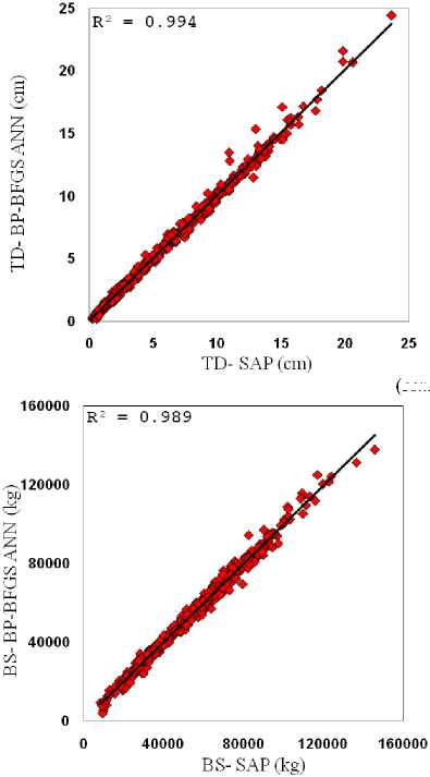
The number of the frames was increased five by five until 150 frames were used. In this step, the number of training and testing pairs were become 1170. At this situation, the prediction results were approach to those of with all studied frames in the previous section, i.e. 427 frames with 3057 pairs. In fact, the optimum number of pairs to training and testing the ANN is 1170. These pairs were also used to train and test the BP-BFGS and BP-LM leading to a novel predicting results which both accuracy and running time were excellent. The final results for the three ANNs, RBF, BP-BFGS and BP-LM are listed in Table 5. It should be noted that the transfer function used for both BP-BFGS and BP-LM was hyperbolic tangent. As shown in the table, the number of epochs is highly reduced compared with the results of the first try listed in Table 4. As such, the elapsed time for BP-LM and RBF are almost 7 and 26 second which is very low compared with those of listed in Table 4. The MSE for both train and test using the three networks is about 0.01% which is very low and acceptable. The MAE results are also satisfactory for both BS and TD, although they are almost equal to those of corresponding results in Table 4. The results of R² are also shown in Fig. 5, demonstrating an excellent correlation between the actual and predicted data. In fact, in this section, an accurate prediction has been achieved by BP-BFGS, BP-LM and RBF networks with rather limited data.

( continued )

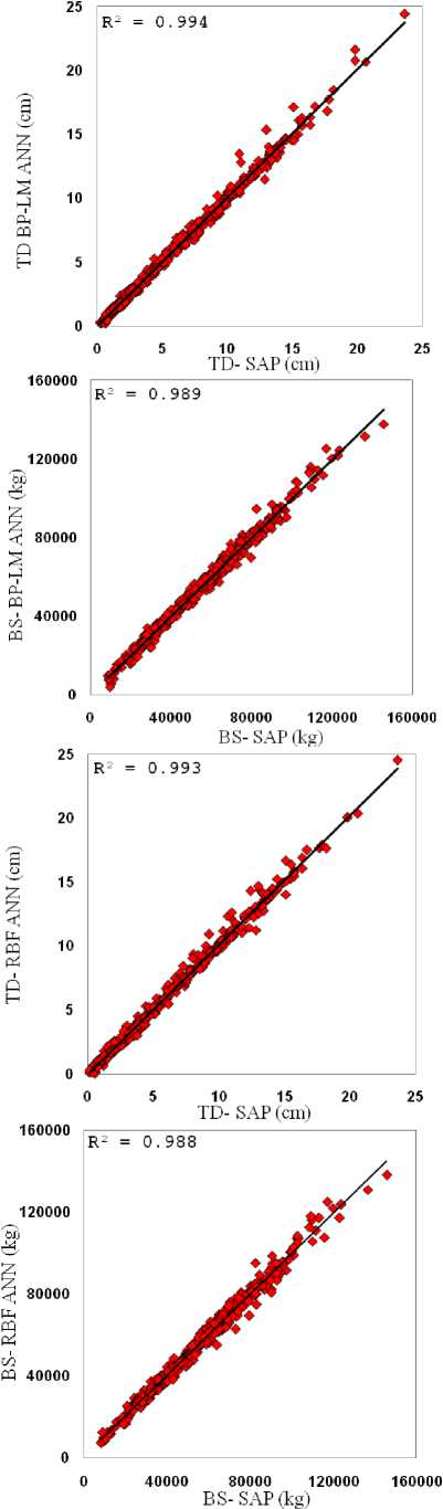
Fig.5. Correlation coefficient for RBF, BP-LM and BP-BFGS based on 1170 pairs.

• VII.    Conclusions

The performance point of semi-rigid steel frames (SRSFs) was predicted by ANNs. Back Propagation (BP) (with eleven different algorithms) and Radial Basis Function (RBF) ANNs were used in order to predict the performance point. Ten input variables including the number of bays, number of stories, bays width, moment of inertia of beams, cross sectional area of columns, cross sectional area of braces, rigidity degree of connections and existence or nonexistence of soft story were used for data generation needed for the prediction. The actual results were obtained at the presence of different earthquake intensity levels and soil types. Three performance metrics of MAE , MSE and R² were used in order to investigate the accuracy of the prediction.

Two trying steps were made in the prediction process. First all the ANNs were used for the prediction including all data samples.

In the second step, three of the best ANNs (in terms of performance metrics) including BP-BFGS, BP-LM and RBF were selected from the previous step. Then, in order to reduce the elapsed time for testing and training steps, it was tried to reduce the number of samples without reducing the accuracy of the ANNs applied. After a trail-and-error process, the number of samples was reduced to from 427 to 100 samples which it was almost 76% reduced. This idea was led to the following remarks:

• •    For BP-BFGS: The elapsed time was almost 70% reduced. The MSE values were almost 4.5% and 11% increased for BS and TD, respectively. The R² values were almost the same.

• •    For BP-LM: The elapsed time was almost 99% reduced which is significant. The MAE values were almost 4.5% and 11% increased for BS and TD, respectively. The R² values were almost the same.

• •    For RBF: The elapsed time was almost 75% reduced. The MAE value was almost 1.2% reduced for BS, and it was almost 9% increased for TS. The R² values were almost the same.

Note that the abovementioned results are for the testing mode. Finally, it is concluded that the performance point of the SRSFs could be accurately predicted by the ANNs used. Among them, BP-BFGS, BP-LM and RBF were the best networks with higher accuracy where the rather limited samples were used.