Prediction of water demand using artificial neural networks models and statistical model

The majority of the countries in the Middle East are suffering problems the increasing demand for water in light of the scarcity of resources to obtain sufficient quantities and satisfy the needs of citizens of different needs in different fields [1]. In general, the water demand and supply depends on the infrastructure of supply, distribution systems, and future strategic plans that have the capacity to meet the needs and sustain the success of the development [2]. So we can describe the Water Demand Forecasting as a total amount of used water, measured or predicted based on a certain application to know the general trend of consumption so as to evaluate the ability of existing resources to meet future needs within a geographic area and to provide the basis for planning future system and improve it to limit the uncertainties for future demand. The water sector is an important sector of sustainable development at the national level. The high demand for water and the significant gap between demand and supply in the water sector is one of the major challenges facing the sector over the next few years. The water demand is increasing because of natural population growth and national development requirements. This is a great challenge, and it is necessary to find creative solutions to supply the necessary quantities of water to different sectors and achieve balance for supply optimal water in Palestine.

The existing models and applications that can predict the water demand effectively is a useful element in strategic planning and the processes of scheduling, maintenance [3]. Prediction strategies of water demand are very important to support and help the water authorities and municipalities in identifying future needs and to develop the necessary plans to find real solutions. The water circumstance in northern Palestine, such as the city of Jenin, is similar to the rest of Palestine cities. But in Jenin city, there are more difficulties back to the amount of water leaking in the ground due to weak of networks and interruptions in supply and consumption during periods. The water department in the municipality of Jenin has no programs or applications for estimating the future demand for water and the calculating and estimating the expected demand is dependent on simple statistical calculation methods, even in the other governorates also there are no modern methods, hence, simple statistical calculations are not enough and not effective and not reliable to provide predicts and estimates that are appropriate for the nature and characteristics of the different regions.

Time series models depend on the premise that any time series have a historical particular recurring statistical that can be manipulated for predict purposes [4]. The unknown time series function F(X t ) to build a model, that allows obtaining accurate predicts [5]. Time series is a combination that represents the data X t , listed and registered over the duration of time for instance, daily, weekly, monthly, yearly, … etc. [6]. Over the years, a wide research effort has been undertaken by researchers to develop effective and powerful models with the aim of improving the possibilities of accurate prediction results. Many models have been developed that predict the time series within the literature in this regard. Stochastic time series models it was used very widely such as ARIMA [7].

Recently, ANNs have increasing attention in the domain of time series prediction, the basic hypothesis to implement this model is that the time series is nonlinear and associated with another parameter known as biologically inspired [8]. The more data and notes are closer to each other over time, the more correlated to each other and stronger.

Different methodologies and methods have been used in the field of water demand prediction in urban areas. These methods depend on statistical extrapolation or advanced analytical models, and the choice of appropriate methodology depends on the purpose of prediction for water service companies and also depends on the quality and quantity of data [9]. Time series prediction is common and the most using is the stochastically style, water demand with time series in the urban areas uses more than form stochastically, autoregressive integrated moving average (ARIMA) models [9]. These models are traditional and linear to the predictability of future values, researches have focused as a tool that has been applied widely in the last decades [10]. Artificial intelligence technique has begun to emerge strongly, especially artificial neural networks (ANNs) and has been proposing as an effective and powerful tool in prediction and modeling [11].

In this work, we will have introduced a different artificial intelligent model based on the artificial neural networks using a learning and optimization algorithms and statistical method, ARIMA model to predict the future water demand in Jenin city depends on the study of the pattern in the historical data. Majority of researches indicate that the water demand prediction with ANNs considers the efficient and strong alternative technique in contrary to traditional and statistical methods [9]. We aim to make performance evaluation of the different methodologies and adopt the most suitable method for water demand prediction in an urban area (case study Jenin city). The actual data that aggregated from the Jenin municipality will be applied as target data for training and input will be the time series of month’s results of consumption. The consumption data was converted to produce 84 values, which present the total water consumption for all subscribers each month. The data is normalized between [0, 1] to fit neural network activation functions that will be used in the applied NNs algorithms and other methods in our work. The applied models (MLPNNs-LM, RBFNNs-GAs, and ARIMA) will produce prediction results for the next year; these models are comparing to select the effective one.

The organization of the rest of this paper is as follows. Section 2 presents an overview of the related work. In section 3, we present the applied statistical model. Section 4 presents the ANNs models. In section 5 we present the proposed applied models for the water demand prediction in detail. Then, in section 6 we show some results that illustrate the prediction result of the applied models. Some final conclusions are drawn in section 7.

• II.    Related Works

Predicting water demand or the needs of consumers in the future or in the short term is one of the main problems facing the management of water distribution systems. Therefore, it is necessary to predict the demand for water with high accuracy and thus reduce the cost. This topic was investigated as shown in the next related work papers which used various methods of neural networks and/or traditional approaches.

Kofinas, D et al 2014 in [9], which provide urban water demand prediction for the island of Skiathos. The authors used four models to predict water demand (artificial neural network, winters additive exponential smoothing, ARIMA, hybrid). The proposed model results compared with all relative statistic of the prediction methods used and thus they deduced that ANNs is the better fitting model according to the root mean square error (RMSE) and others parameters like high (R square) represent how close the data are to the fitted regression line. In [10] the authors proposed three different modelings to prediction water demand for the optimal operation of large-scale drinking water, they employed a Seasonal Auto-Regressive Integrated Moving Average (SARIMA) model, a Box-Cox transformation, ARMA Errors, Trends and Seasonality (BATS) modeling, and an RBF-based Support Vector Machine model. They established time series modeling methodologies and employed it to capture the dynamics of water demand, these models are trained using the same dataset, and the models are statistically validated of their prediction error. All models proved to be appropriate for the estimating of the demand.

Deng, Xiao, et al. in [45], the authors introduce a new approach namely a hybrid EEMD-Elman neural network model to predicting the hourly campus water demand, they are combined the Elman neural networks (ENNs) and

Empirical mode decomposition (EMD) method and carried out the prediction of water consumption hourly for 31 days on the campus of Hebei University of Engineering. The actual water consumption and the predicted results were carried out over the EEMD-improved ENNs model and compared with the single Backpropagation (BP) and ENNs, the results indicate that the combined model has a good performance in prediction hourly water demand and achieved minimum error and more accuracy but the complexity was increased.

Xing, Ying, Zhenwei You, et al. in [44], improve the new way of back-propagation (BP) by means of two heuristic algorithms, they developed the back-propagation by combining it with genetic algorithms (GAs) and particle swarm optimization (PSO), in order to do real-life water demand prediction of Beijing city, they tried to increasing the accuracy of prediction process by the testing and verification of the three algorithms (BP, BP with GAs , BP with PSO). Although the execution time consumed is taking longer time but both BP with GAs, BP with PSO performed with higher accuracy and less errors than BP algorithm.

A new technique of ANNs called water demand to predict (WDF) is proposed in [14] to modeling and prediction the water demand in urban areas, the study area was chosen in Weinan City in China that consists of 9 years of data. Authors developed a simple ANNs model consisting of only one hidden layer with the BP algorithm, the authors are deduced according to analysis and results that the approach of ANNs displays the possibility to estimate and formulate water demand for home use in an efficient way. The proposed model shows that the correlation coefficients are more than 90% both for the training data and the testing data.

Memarian Hadi, Siva Kumar Balasundram in [41], introduced the predictive performance of the Radial Basis Function (RBF) and Multi-Layer Perceptron (MLP) to predict the sediment load in a tropical watershed. Time series data of daily sediment discharge and water discharge at the Langat River, Malaysia obtained from 1997 through 2008 recorded were used for training and testing the networks, The MLP was trained by a backpropagation algorithm, for transfer activation function the logistic function and the hyperbolic tangent are employed and each weight in the network was adapting by updating the present value by gradient descent learning algorithm, the authors applied the same datasets for network training and testing in both types of network, so they divided data by employing 54% for training and 14% for cross-validation and the rest of the data equal 32% is employed for Network testing. The experimental result indicated according to the minimum MSE obtained of the RBF network was larger than the MLP network and the MLP network achieved the best-fitted output to the cross-validation data set than the RBF network. Also, MLP network in testing data achieved the lowest MSE and NMSE when compared with RBF network, add to that the MLP network showed additionally qualified in term of depiction the fluctuations in daily sediment load than the RBF network.

JAIN, et al. in [42], The ANNs, regression, time series analysis technique, have been examining to model the short-term water demand predicts, precisely two-time series models, five regression models, and six ANNs models, where progressing and developing. All the above models were carried out to select the appropriate of each technique investigated to model water demand predicts. According to the results gained in this study and the comparative analysis, it has been shown that the models of ANNs technique have performed better than the models using classic and traditional techniques of time series analysis and regression, so the complex ANNs model performed the best among all the models developed in this study.

Ishmael S, et al. in [43], Two machine learning techniques have been used and tested in this paper, the artificial neural networks and the support vector machines are used to predict short-term and long-term water demands, two types of neural networks architectures is used, MLPNNs and RBFNNs, SVM experiment was including of many models, the models were compared to each other in order to locate the Support Vector Genius (SVG). The result produces that artificial neural networks perform prediction result better than SVM.

In this paper, different models of neural networks and statistical are used to predict the water demand in next year depending on the pattern of the demand in the previous data. The aim is to create a model capable of making an accurate prediction for water demand in the future for the Jenin city. Two applied models of ANNs are used; MLPNNs-LM and RBFNNs-GAs, and one type of linear statistical method called Autoregressive Integrated Moving Average (ARIMA) are applied.

• III.    Stochastic Models

A widespread statistical method vastly used to foresee the time series is the ARIMA model. ARIMA is a term (concept) and expression that stands for Auto Regressive Integrated Moving Average; it is a manner and paradigm that captures a set of different temporal component in time series data, ARIMA is a prediction method that visualizes the future values of a certain series, others call it “Box-Jenkins” [12]. ARIMA is commonly better and more efficient than the exponential smoothing method given that the length of data is moderately and the observations of time series are stationary or stable and the correlation between these observations must exist [12, 22].

SARIMA is another type and it similar ARIMA but the first take into account the seasonality issues, thus we can demonstrate the model as ARIMA add to that the part of seasonality (P, D, Q), so the adopted form is by employing the following expression: (p, d, q) X (P, D, Q). Many applications provide us with the possibility of building ARIMA models such as MINITAB, MATLAB, IBM-SPSS-STATICS, and the most professional is the R-studio, which provides us with ready tools to shorten the long list of procedures, calculations, and representations and suggest to us the best usability. Actually, ARIMA suffering from some limitation, such that the ARIMA method is dealing just with a linearity shape, and it suitable with only for a time series that is stationary, this means that it is variance and mean must be a constant through the time [7, 24], add to that they need a large number of observations to be an efficient manner, So the accuracy of forecasting according to this manner is mostly a variable especially if they represent a linear manner for nonlinear problems.

• IV.    Artificial Neural Networks

The Neural Network in term of biological status is imitating the human brain. The brain, in general, depends on a small processor of nerve cells, which are called neurons or nodes. The ANNs consisted of a number of simple processors, called neurons, which are approximately similar to the biological neurons in the brain. ANNs have been characterized by many reasons and that makes them very suitable for particular problems, so it has the ability to learn, generalize, does not force any limitation on the input for variables, especially in the complexity observations in predicting, unlike traditional models, it ready to be the powerful alternative technique.

ANNs are basically developed to mimic the human brain, a non-linear calculation executes through neuron according to the input values and perform result values to transfer and fed others neurons, in more clear shape every neuron obtains the input signal or total information from another neuron, the processing is done through activation functions to generate a converted output signal to other nodes and exterior outputs. It should be noted that although each neuron performs its function somewhat slowly but the network in a collective and participatory way progress the huge number of calculations and processes in a manner of high speed and high efficiency [13].

The advantages according to a wide range of parallel distributed processor makes ANN's strong arithmetic tools and enormous in computation, the greatest achievement is the enormous ability to learn according to data situations and initial observations and then produce and generate new cases and examples that haven't seen before, NNs learns depends on the input data and the related output data, hence this is known as the generalization ability of the ANNs [14]. In general, the past observations of the data series represent the input, as for the future value represents the output and the ANNs calculate this as this function:

X t _{+ 1} = F ( X t , X t - 1, X t - 2,..., X t - n ) (1)

Where X is the observation at time t, neural networks in terms of topology can fall under two categories where there are networks with a single layer and there are networks that can contain multiple layers. It is important to note the important aspect of the flow of data (the feedforward or feedback neural networks), but the central part of the whole process is the subject of learning algorithms, which plays a pivotal role in intracellular communication between neurons to determine and adjust weights. The learning process has two kinds, the supervised and unsupervised. Every artificial neural network consists of several compounds: a set of x as an input vector that represents the values that are pass-through nodes to the hidden layer. So every node from the input layer to the hidden layer takes a random weight w value, thus it is an actual value that concise together with an input value to the neuron. At all neuron within the hidden layer, we employing the transfer function that grants propagating of output to the rest of the neurons [15] and figures 1 show some explanation, it is worth mentioning here that the network has the ability to learn, by adjusting its interconnection weights.

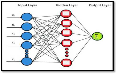
Fig.1. Basic Artificial Neural Network

Often, single layer Perceptron cannot solve some of the complex problems, so we need more efficient and effective methods. The importance of the hidden layer is that it receives the input through the neurons and analyses it with the aim of making the appropriate decision about what to do according to the acquired experience and learning [16], Then is passes it to the rest of the neuron cells and nodes through communication after the recruitment and implementation of certain types of activation functions such as the (sigmoid) [17]. This means that neural networks have high capabilities in adaptive learning and training processes. So the network possesses the characteristics of self-organization in order to achieve the desired goals. The output values are calculated and produced and passed to the output neural network layer at the end. Hence we can express the output by employing the following equation.

m

Y = f ( Z W j X j + b i )             (2)

j = 1

Where Yi is the network output, wij are the weights, xj is the value of a set of inputs, m is the total number of inputs, bi is the bias, often enclose as additional weight, essentially it equals 1. Extraction the value of the error is a process carries through back-propagation, so the network calculated the error between the target value and the calculated output value knowing that the weights are updated by employing some training technique and all this process, the network is reiterated until we obtain the satisfy minimize network error, the error is basically calculated using the following equation:

e p = ^Yp - Y d( p )                     (3)

Where Y(p) is the target and Y_d(p) is the desired output. We must note that the weights in the first stage are random, according to the error propagation, the weights continue to adjust until the error criteria are satisfied according to ϴ, and ϴ is the threshold value of the prediction process. Typically, in the prediction process, there is a basic rule of stopping training through a prior condition, in our paper we employing the mean square error value (MSE), the following expression presented it [18]:

MSE = ^ ( T arg et - predict ) 2 / n <  9       (4)

Where n is the number of inputs.

MLPNNs and RBFNNs have been applied successfully to predict or approximate some difficult and complex problems by training them in a supervised manner with the using of robust algorithms. In our paper, the Multilayer Perceptron Feed Forward NNs with Backpropagation process and Radial Basis Function NNs with Genetic algorithm consists of three layers are proposed to optimize the connection weights, so it is generally the mostly applied in ANNs.

Regardless of the models used or methodologies adopted and applied remains the main objective of a time series is to construct a model to infer future unknown data from existing data by reducing the error between actual and desired values. Many methods have been proposed over the past years to assess future needs and have been investigated in several areas, domains, and fields. In the following sections, we will review in detail the methods that have been investigated and applied in this paper

The water demand prediction in this work depends on the historical data, thus required data were extracted mainly from the municipality of Jenin city database management system. The dataset used in this paper consists of recorded water consumption parameters in the Water Department which follow the municipality of Jenin city. The dataset was extracted and obtained for the last seven years according to the period between 2011 and 2017, we aggregated the total consumption for instance in one month for 7500 customers so as to obtain just one value that represents the total consumption vector for all customers in one month in year, hence we obtained the 84 values represent 84 months and thus represent 7 years, this data used and exploited on all models intended to be built and implemented.

The total consumption vector for each month individually converted and normalized to the range between zero and one to facilitate the computation process according to the following equation:

• V.    The Proposed Applied Models

In an attempt to build models, systems, and applications in order to estimate the future needs of something, it is necessary to take into account the amount of accuracy that will be achieved. Therefore, the decision to build models for the future prediction of water needs to be as accurate and reliable as possible so as to produce and choose the best one. Water demand prediction based on reliable modeling and predictability of the future has received considerable attention from researchers at the global and regional levels because of the vital role in the future strategic planning process. In Palestine, the applied methods depend on simple statistical or numerical ways. The primary objective of this work is to establish a more applicable artificial neural networks model or other traditional methods that can be used to predict water demand in the short-term period in order to help to achieve water resources sustainability. Prediction the future water demand depends on extract the patterns of the historical demand data, the data set was collected from Jenin city in the north of Palestine as a case study. We apply a general statistical ARIMA model to predict water demand value in the short term period (next year), and also we employing and apply a more efficient artificial neural networks models with different learning algorithms to predict the water demand in a short-term period, add to that we studying and comparing the different applied models depending on their architectures and the prediction result (smallest MSE) to determine the best model for predicting.

_{Y =}    ⁽ X - miⁿ⁽ x ))

• ¹   (max( x ) - min( x ))

  
  

Where x i is the actual consumption and y i is the normalized value, min and max are the maximum and minimum values for actual consumption [19]. Figure 2 illustrated the general procure of the applied models. In the next sections, we will present in detail these applied models.

From figure 2, we find that architecture passes and consists of several stages. Initially, all dataset is stored in the municipality database, this data stored in several different formats where it must pass by process of converting data or information from one format to another, data that meaningless is dropped and deleted, this includes any data that cannot be understood and interpreted correctly by machines

Data normalized to organizing data in a database belonging to us, including the creating new tables and redesign relationships between those tables and then to convert all water consumption values to range between zero and one to facilitate computation process. The cross-validation it’s necessary for any non-linear neural networks techniques by separate the data to have a training set and testing set in order to verify and to check its validity and estimate the quality of the models, the next is training and testing the time series of all models (ARIMA, MLPNNs, RBFNNs), also executing the prediction according to all models in order to obtain the results.

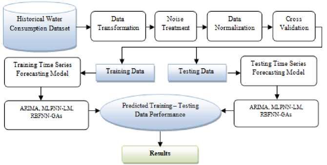
Fig.2. General Procedure

• A.    ARIMA Time Series Predictor

Autoregressive Integrated Moving Average, (Box-Jenkins) and multi-linear regression models have been broadly implemented in various predictions in many fields, such as financial, industrial, commercial, climatic and demographic fields, but accuracy is a variable because they represent a linear manner of nonlinear systems [20].

As such, the use of the ARIMA model is proven to be effective in demand forecasting technology. Numerous mathematical time series forecasting approaches, like exponential smoothing, assume that every data point in the time series values will consist of the deterministic mean and a random error. Most often time series characterized by a large grade of dependency between sequential observations. So the time series of water demand giving such dependency between observations because of a great daily, weekly or monthly cycles inside the consumption patterns, hence the ARIMA forecasting manner is intended to benefit from this dependency in order to create the prediction. The technique of ARIMA must achieve many essential components, so the components are:

Autoregressive (AR), it is a time series paradigm use the past observations as input to feed a regression equation to predict the value in future vision, based on a linear combination [21]. For instance, we can predict the values for a later time t+1 by given two times of past observation t-1, t-2 as a regression model by employing the following equation:

x ( t + 1) = b₀ + b 1 * x ( t - 1) + b 2 * x ( t - 2) (6)

Where [b0, b1, b2] are coefficients obtained through optimizing process on training data, It represents the value and amount of the regression slope of the dependent variable on the independent variable and X is representing the input. Integrated (I): it finds the difference between the observations that represent the actual and raw data, In other words, we subtract the current observation from previous observation [22]. Differencing is a very good way of change or converts a non-stationary time series to another stationary. Basically, this approach can remove the trend if we saw that the rising time series is rising at a fixed rate. In this way, we can apply only once, this is called “first differenced”, mathematically as an equation.

Yt = Yt - Y ( t - 1)                 (7)

If achieved purpose of making the curve of time series is stationary and the trend was removed then the first-differenced will be enough, if not we can repeat the procedure again and this called “second differenced”, mathematically as an equation.

Y * = Yt - 2 Y ( t - 1) + Y ( t - 2)            (8)

Moving Average ( MA ): determine that the output value relies in a linear way on the current value and previous values, this model uses the dependency among the observation and between lags of the predicted error in moving average approaches [23, 24]. In other meaning, each value of X (t) is immediately linked just to the random error in the past E (t-1) , and to the current error E(t), so the subsequent equation represents it:

X_t = ц +S t + 9 1 Z ( t - 1) +...... + 9 q Z ( t - q )     (9)

Where µ : mean of the time series, Ɵ : parameters model, Ƹt_, Ƹ_t-1, Ƹ_t-q: white noise error represent residual errors series x_t and represent the difference between an observed value and a predicted value from a time series model at a particular time t.

In general, select the best model of ARIMA and the model order is not easy, and the user must have a good experience and high level of skills because of ARIMA model includes a large number of details and the statistical equations. ARIMA model consists of three component or parameters, non-seasonality (p, d, q), where; p: represent the lags of stationeries series (AR), the order of non-seasonal (AR); we determine it through partial autocorrelation function (PACF), d: differencing between the observations (I), and q: represent the lags of the predict errors (MA), the order of non-seasonal (MA), we determine it through autocorrelation function (ACF). SARIMA is another type and it similar ARIMA but the first take into account the seasonality issues, thus we can demonstrate the model as ARIMA add to that the part of seasonality (P, D, Q), so the adopted form is (p, d, q) X(P, D, Q).

The expert statisticians Box and Jenkins [25], in (1970) establish a practical approach to create the ARIMA model, which given the best match to time series. This approach has an essential significance in the domain of time series analysis and forecast [26].

The Box-Jenkins technique is based on the assumption that there is no particular pattern in the historical data of the time series to be predicted. But the alternative is to use a three-step iterative approach of model identification, parameter estimation, and diagnostic checking to determine the best model from a certain number of ARIMA models [27]. The process is repeated continuously many times until an accurate model is finally discovered, and then this model can be used for predicting future values of the time series.

To provide the practical approach of Box and Jenkins in order to build the models of ARIMA we must go through multiple stages starting from fetching data and ending with the adoption of a predictive model that achieves the goal.

First stages are called identification, we aim at this stage to determine the order of the model wanted ( p, d, q ) so as to take and know the data properties and the major features of series, such that capture the trend both (increasing/decreasing), also the series is (stationary-non-stationary), add to that to determine seasonality or not for the time series according to use graphical procedures (plotting the series, ACF/ autocorrelation function and PACF/ Partial autocorrelation function). So a time series must be stationary and it is “stable”, that means the mean is constant over time (there is no trend) and the correlation structure between every point in the time series remains constant over time, so we always demanding to remove the trend and seasonality in order to move on to the next stage.

Hence the ACF plots can help us to determine the order of the moving average (MA) ( q ) model, add to that the PACF plots areas very significant role for determining the order of the Autoregressive (AR) ( p ) model. The next stage is called the estimation and diagnostic checking to determine and selection the best model, which includes the estimation of the parameters of the several models using previous stage and produce the first best selection of models based on (whether using the Akaike Information Criterion AIC or the Bayesian Information Criterion BIC) [28][29], it is widely used to measure the goodness fit in any estimated statistical model, and which are defined below according the equations [28]:

л 2

AIC,„) = n In ( -^) + 2 p (10) pn л2

BICp == n ln( ——) + p + p ln( n ) (11)

Where ( n ) is the number of observations to fit the model, ( p ) is the number of parameters in the model and (σ) is the sum of sample squared residuals. The best model order is picked by the number of model parameters, which minimizes either AIC or BIC [12]. The final stage is called the diagnostic. In this stage, we are concerned about three issues; first is (P value for Ljung-box statistic) and this means that all values of (P-value) must be higher than 0.05 and therefore we do not reject the initial hypothesis that indicating that the model meets the purpose.

The second issue is ACF of residual, we concern about the violation if exist, else that our assumption for adopted model stay meets our need. The final issue is standardized residual and must care about the randomization that does not indicate to the pattern, so we don’t need for any pattern, add to that there is additive diagnose include the observance of normality. Based on all stages above, we can carry out the predicting, it is applied step to produce the prediction based on the model you decide is best.

The title of the paper is centered 17.8 mm (0.67") below the top of the page in 24 point font. Right below the title (separated by single line spacing) are the names of the authors. The font size for the authors is 11pt. Author affiliations shall be in 9 pt.

• B.    Multilayer Perceptron Neural Networks

Predicting the future demand for water consumption in many areas was performed according to the numerical models, statistical methods, and time series prediction based on the applications of statistical linear and nonlinear techniques. The basic rule of Multi-Layer Feed Forward Network is that all connections flow in one direction, meaning that the data is streaming from the input layer to the output layer. On the other hand, the Back Propagation Network is a type of gradient descent mechanism with backward error propagation [30]. Comparisons continue between the initial outputs of the network and between the real values by modifying the network parameters repeatedly and continuously to obtain the lowest error value, the greater the amount of data available, the higher the performance of BPN. In recent times, according to the results of experiments and practical practices and the use of various statistical and traditional algorithms, artificial neural networks, especially multilayer Perceptron, are very effective and powerful and alternative to other methods, unlike traditional statistical methods, multilayer Perceptron does not care about any prior assumptions about data distribution or relationships between them.

A major issue and feature are that it has non-linear functions and can be trained to accurate generalization when presented with new unseen data [30]. A multi-layer perceptron network is capable of creating an approximation of any function and smooth, it is a measurable function between input and output vectors depending on the appropriate choice of weights and connections [30]. Multi-layer Perceptron depend on the supervised way to learn, The applied procedure to execute the learning operation in NNs is called training Algorithm

[31], through the training may be the results not equal the desired output, so the error is calculated and this error belonging to variation between the desired and actual output. Thus the training uses the size of this error signal to decide the degree of weights must be adjusted or modified, hence we obtain the lowest error of the Multilayer Perceptron. Optimizing and adjusting the weights is the core of the training process in multilayer Perceptron which determines through it the feasibility and ability of the network to give us the optimal solutions about a certain problem in an accurate manner. The most important training algorithms that are known for Neural Networks are (Gradient descent [32], Newton's method, Quasi-Newton [33], Levenberg Marquardt algorithm [34]) algorithm. In our paper, the Multilayer Perceptron feed-forward with a back-propagation neural networks model is adapted to predict the future demand for water consumption. Our proposed model according to Multilayer Perceptron Feed Forward with Back Propagation Neural Networks depends on the following steps:

• >    Input: dataset consist of the time series of 84 data points >  Output: prediction of future water demand result DATA PREPROCESSING:

• ❖    Normalize (input time series, target)

The Initialization process can be done either by fixed weights or random, in our case we used random initialization.

• ❖    Determine input pattern X_t: (X_t1, X_t2... X_tn )

• ❖    Determine target output from the collected data

Feed Forward Phase:

Firstly, calculate the predicted output of the first hidden layer ( out L1 ) by employing the sigmoid activation function ( f ¹ ).

n outL1 = f 1£ Xi. Wli)             (12)

i = 1

f ¹ =

1 + e - ^x

This predicted output of the first hidden layer ( out L1 ) will be the input of the second hidden layer ( Y ), and then we calculate the predicted output for the second hidden layer ( Y ) also by employing the activation function ( f ² ).

n

Y = f ²£ out_u. W jL 2 )            (14)

j = 1

f ² = X                 (15)

Between the target data and the output of the network, there are some errors which we aim to reduce it to a little as possible.

Backward phase:

Calculate errors using the expression:

N

V E i =<- = ^Ja¹ , ( y ‘- y_t )        (16)

e w

Where E is the error function, J is the Hessian matrix calculated as:

N

J j = Z

= 1

^{d y} 5 y d w i d w

⁺ ^ I M

Where I M is the identity matrix of order M , and λ is a parameter that makes a function similar to learning in the back-propagation algorithm, w ⁱ is an i ^th element of input layer weight, w is a j^{t h} element of output layer weight,y / is the derivative output of l^th the neuron, у / is output of the l^th the neuron.

Update weights:

The modification of the weights with the Levenberg-Marquardt method in the μi ^th learning cycle starting with the output neurons and backward until reaching the input layer by the following expression:

W ( p ) = W ( p - 1) - J ^-x( p - 1) V E ( p - 1) (18)

The general process for Multilayer Perceptron Feed Forward NNs with Back Propagation is illustrated as shown in figure 3:

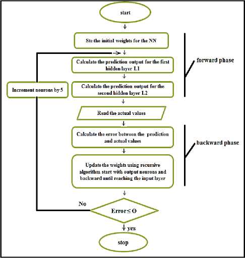
Fig.3. MLPFFBP General Process.

C. Radial Basis Function Neural Networks

The main idea of RBFNNs is originated from the theory of function approximation [36]. The network was designed by the Darken and Moody (1989) and the network depend on two layers other than the input layer, namely, hidden and output layers. This network converts inputs in a nonlinear way and finds the appropriate curve to give the correct results. The network is feed-forward and contains two types of learning methods of neural networks, so that the learning between the input layer and the hidden layer is unsupervised and the data is grouped into totals between the input data and the weights of the hidden layer that are initially randomly selected without the need to know the output, in this layer the activation function Gaussian Radial Basis Functions is used.

The learning between the hidden layer and the output layer is supervised and depends on the degree of error on the outputs. The hidden layer of RBFNNs is nonlinear and the output layer is linear, whereas the hidden and output layers of MLPNNs are usually nonlinear [35].

One feature of the RBFNNs is that any function of a limited range can be approximated by employing a linear combination of radial basis [23, 36]. The radial basis function network consists of three layers of nodes; these layers are the input layer, hidden layer, and an output layer. Each layer in this network is connected with the next layer, meaning that every node in the input layer is connected to all the nodes in the hidden layer, and the hidden layer nodes send their outputs to each node in the output layer. The number of nodes in the input layer depends on the application given to the network, and the number nodes in the hidden layer depend on the complexity of the given application (issue), the following figure 4 illustrates the three-layer radial base function network.

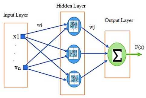
Fig.4. Radial Basis Function Neural Networks Structure

Note from the previous figure that each node in any layer is connected to all the nodes of another layer by means of weights w , the input of the network is represented by a vector x and the output of the network is F ( x ) and n is the dimensions of the input data.

The output of the neuron in the output layer of an RBF Network, where is given by [37].

m f (x,Ф, W) = ^ фi (x ).w,.              (19)

i = 1

Where ф is the activation of the radial unit for the input pattern x and w_i is the weight between the radial unit i and the output neuron m [38], the activation of the i ^th radial unit is dependent on the distance between the input pattern and the hidden unit center, using an Euclidean metric [39], In the hidden layer, the activation function used as a Gaussian, the activation of the i ^th radial unit can be defined as using the following mathematical form [37]:

ф ( x , c , r ) = exp |           |                (20)

к r )

Where c is the central point of the function ф , r is its radius and x is the input vector.

RBFNNs also have own training algorithm as a Gaussian training algorithm, also many methods proposed such as employs the K-Means clustering (KMC) algorithm to determine the RBF centers location, Also employed the K-nearest neighbor’s technique (KNN) to optimize of the radius of each RBF radius, and singular value decomposition algorithm used in RBFNNs for optimization of weights matrix of the output layer. A recently genetic algorithm is presented by optimization of its topology includes the parameters (centers, and radius), so the possibilities of employing GAs to configure an RBFNNs exists and available.

In our paper as an RBFNN, the training procedure is divided into two stages [37, 40]. First, the parameters centers and radius of the hidden layer are determined by genetic algorithms (GAs). Second, the weights connecting the hidden layer with the output layer are determined by the Singular Value Decomposition (SVD) algorithms method is adopted. In [37], a common approach presents several ways that depend on optimizing the topology of RBFNNs and parameters centers c , radius r using GAs, weights w calculated by means of methods of resolution of linear equations, in this algorithm the author used the singular values decomposition (SVD) to solve this system of linear equations and assign the weight w for RBFNNs to calculate the output. In our paper, we adopted the same approach. The principle of the work according to this integration algorithm as follows; In the beginning, we must note that each individual of the population is composed of two real vector parts representing the center and its real values, also represent the radius, so we can visualize the individual (chromosome) contains variable lengths as this series

[ c 1 \ ^r 1 , c ₂\ Г , ,....., c n \ r n ]                ⁽²¹⁾

We get the initial population of ( c : canters, r : radios) randomly by using a number of certain individuals, note that each individual length depends on the number of RBF (number of a neuron). The Singular value decomposition

(SVD) used immediately to optimize the weights. Now the c: canters, r: radios and also the w: weight become ready, and we can find and calculation the output of RBF network, for the evaluation function, it is the tool that measures the value of the fitness in each chromosome, so we consider the mean square error between the actual output and the predicted output is the fitness function [37].

In order to stop the algorithm, we used the criterion of the upper limit of the generation. So when the genetic algorithm moves from generation to generation and before approaching the upper limit of the generation without significant changes in fitness values, we end the process. Many methods can use to do individuals selection, in this methodology the Geometric Ranking method was adopted, so the following equation explains it [37, 40]:

p [ individual 1 selection - i ] = d ⁺ ( 1 - d ) r 1 (22)

• ❖    Get an initial population of (c: canters, r:  radios)

randomly by using # of certain individuals

V Each individual length depends on the number of RBF [c1|r1, c2|r2… c n |r n ]

• ❖    Calculate the output of (RBFNNs) using

m

f(x,ф, w) = ^ф(x).w i=1

• ❖    Calculate the MSE of (RBFNNs) using

.2 ,

(T arg et - predict ) / n

❖ Apply selection using the Geometric Ranking method using

d+

d

1 - ( 1 - d ) s

p [ individual 1 selection - i ] = d ⁺ ( 1 - d ) r ¹

d+

d

1 - ( 1 - d ) s

Where d is the probability of selecting the best individual, r is the line of the individual, where 1 is the best; the s is the size of the population [37]. The crossover using to produces two new individuals as in the following equations:

x = rx + ( 1 - r ) y

Where d is the probability of selecting the best individual, r is the line of the individual, where 1 is the best; the s is the size of the population

• ❖ Apply crossover to produces two new individuals using

x=rx+(1-r) y y=(1-r ) x + ry                (25)

y = ( 1 - r ) x + ry

Where ( x and y ) are two vectors belonging to individuals (parents) of the population, r is the probability of crossover between ( 0, 1 ) [35]. The uniform mutation is employed to select one element randomly according to the following equation [37]:

,  JU (ai, bi): fi= j x‘ =1       ,

[ X i otherwise

Where a and b are down and the top level for every variable i .

Every step we increase the number of RBF and continue to repeat the process until the number of iteration less than the generation number or less than the threshold (errorrate). Our proposed model according to RBFNN-GAs depends on the following steps:

• > Input: Dataset consist of a time series of 84 points >  Output: prediction the future water demand result ❖ Data processing:

• •    Normalize (input time series, target)

• •    Initialize the weight W of RBFNN using SVD

• •    Determine input pattern X_t: (x_t1, x_t2, ..., x_tn)

• •    Determine target output from collected data

Where ( x and y ) are two vectors belonging to individuals (parents) of the population, (r) is the probability of crossover between (0, 1)

❖ Apply mutation to select one element randomly

,  JU (a„ bi): fi= j x‘ =1

[ X i otherwise

• ❖    Increase the number of [RBFs]

• ❖    Repeat

• ❖    Stop if the number of iteration less than generation number or less than the threshold (error rate)

• VI.    Experimental Results and Discussion

  In all experiments procedures and applied models which we have designed, we tested them by employing the MATLAB R2013a and R-studio (R language) under Windows 7 with Core i3-M 380 CPU 2.53GHz, 4GB RAM memory. We intend to offer the outcomes that were produced in the practical experiments of our predictions by providing numerical and graphical results according to the monthly prediction based on all models that we developed and constructed. After that, we intend also to offer the

comparison and the results of all models and experiments between different neural networks and the ARIMA model. We provide the monthly prediction results for Multi-Layer Perceptron Feed Forward NNs with Back Propagation Algorithm, RBFNNs Models with Genetic algorithms to optimize the canters and ARIMA Time Series Predictor using Box-Jenkins Methodology.

• A.    Monthly Prediction (ARIMA- Box-Jenkins) Methodology

  To prediction the water demand for the future according to Box-Jenkins Methodology, we must pass through many stages, so at the beginning we convert the actual consumption values over seven years starting from (Jan-2011) to (Dec-2017) to normalized data format, so that all values will take place between the value of [0,1]. We obtained 84 value represent 84 months to prediction a new 12 months that represent the year of 2018. After we explore the major features of series such that captured the trend both (increasing/decreasing), also the series is (stationary-non-stationary), add to that determined seasonality for the time series according to used graphical procedures (plotting the series, ACF/ autocorrelation function and PACF/ Partial autocorrelation function). So we made a time series is stationary and it is “stable”, hence we removed the trend and seasonality in order to move on to the next stage, figure 5 depicts this procedure.

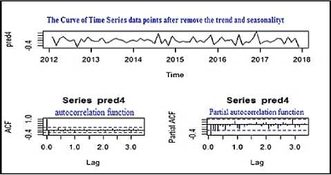
Fig.5. graphical procedures for a stable time Series after removing the trend and seasonality

According to the ACF plots we tried to determine the order of the moving average (MA) (q) model, and according to the PACF plots we tried to determine the order of the Autoregressive (AR) (p) model. To estimate and diagnostic checking stage we have determined and selected the best model including the estimation of the parameters of the several 10 models using the previous stage and produce the first best selection of models based on the Akaike Information Criterion AIC and the Bayesian Information Criterion BIC. Since we repeated and tested more than one model, we were careful about three issues; the first is (P value for Ljung-box statistic) and we sure that all values of (P-value) is higher than 0.05 and therefore we don’t reject the initial hypothesis that indicating that the model meets our purpose. The second issue is ACF of residual; we sure about the violation not exist, so our adopted model stay meets our need. The final thing is standardized residual and we also sure that randomization does not indicate to the pattern, figure 6 depicts that.

Cross-validation model is carried out by partition the data into two subsets; the training set will use the majority of the data. The larger amount of data is used to set up a model in training. For our dataset is divided into two sets, 70% for the training set and 30% for the testing set. So figure 7 depict this.

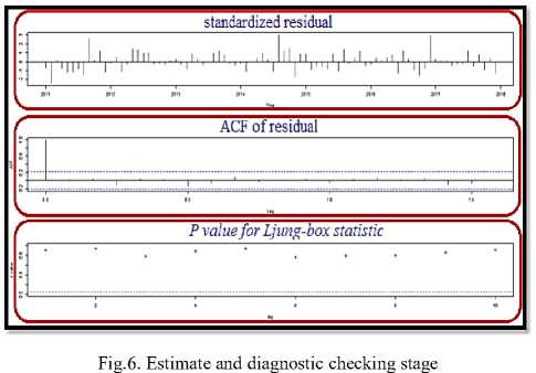
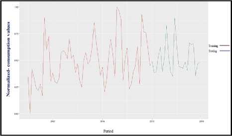
Fig.7. ARIMA Cross-validation model

Based on all the above stages, we carried out the prediction, this step is applied to produce the prediction according to the model that we are decided is the best one. Here we intend to generate a new 12 months that represent adding one year (2018) and then present the results that the ARIMA model returned to be compared later with the rest of the methodologies used in this thesis, so figure 8 illustrate the prediction process.

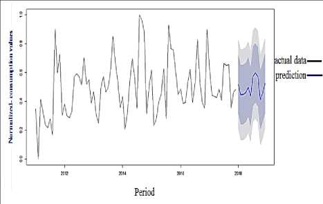
Fig.8. ARIMA best prediction result for 2018

According to what we have the dataset that we mentioned in previous places and other section in this thesis. As we have seen in the figure we carried out the prediction based on the R-studio, we built a special and specific model for our problem, ARIMA tried to produce the best results and do the best effort based on the error in training, testing values, and the fitting. The best root mean squared error (RMSE) was obtained is depicted in Table 1.

t able 1. b est root mean squared error (rmse)

Training set (RMSE)	Test set (RMSE)
0.1696096	0.2257397

That means that the mean squared error for training is (MSE_train = 0.028) and the mean squared error for testing is (MSE test = 0.051), Knowing that MSE = (RMSE)². In a more graphic way, we can see the comparison produced by the ARIMA model between the actual data representing the test data that came from reality and the prediction values according to the model adopted, so figure 9 illustrates this.

From the results of month’s prediction as in table 1, and figures 8 and 9, it’s clear that the proposed ARIMA model produces some good results in some extent based on the mean squared error of training and testing sets that obtained for the future prediction of water consumption demand.

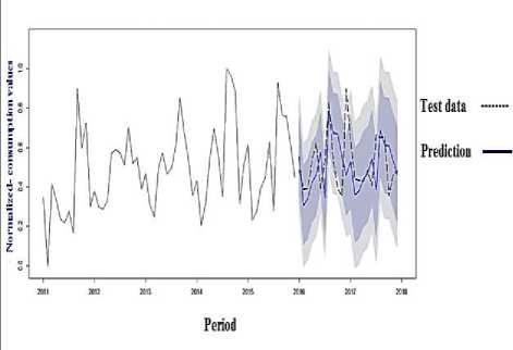
Fig.9. Comparison between reality and the prediction values

• B.    Monthly Prediction (MLPNNs-LM

  To predict the water demand in monthly style, we compute the total consumption, for instance in one month for 7500 customers so as to obtain just one value that represents the total consumption for all customers in one month in the year, hence we obtained the 84 values that represent 84 months and thus represent 7 years. We use the MATLAB R2013a to produce the predicting, the outcomes of values are given a number of neurons that represent the series of neurons used in every Multilayer Perceptron Feed Forward Back-propagation, number of Iterations that represent the number of the execution cycle of every Multilayer Perceptron Feed Forward Back-propagation, mean squared error for training (MSE train ), mean squared error for testing (MSE_test). Cross-validation model is

carried out by dividing the data into two sets as we do the same thing for this Methodology, so each set is a percentage value as 70% for the training set and 30% for the testing set.

Table 2. MLPFFNNBP (monthly water demand Prediction Result)

No of Neurons	MSE train	MSE test	No of Iteration
5	3.22535E-02	4.38334E-02	8
10	2.81714E-02	4.49053E-02	13
15	1.71894E-02	3.98097E-02	8
20	1.87715E-02	3.33202E-02	8
25	1.66460E-02	2.95369E-02	8
30	1.26527E-02	4.82637E-02	7
35	1.35805E-02	3.09674E-02	8
40	1.29510E-02	2.03809E-02	7
45	5.43525E-03	3.88319E-02	8
50	7.37251E-03	8.79243E-02	8
55	1.28419E-02	3.82644E-02	7
60	5.91304E-04	3.35725E-02	8
65	3.19636E-03	6.79492E-02	7
70	1.86360E-03	1.00880E-01	8
75	8.28180E-03	1.29360E-01	5
80	3.81429E-05	1.46403E-01	6

Table 2 shows the mean square error values and iterations number of training and testing incrementally starting from (5) neurons to (80) neurons by increasing (5) neuron in every cycle. According to table 2 and figure 10, it is clear that the Multilayer Perceptron Feed Forward NNs with Back-propagation LM approach made a very good result for the prediction according to an appropriate quantity of neurons in the hidden layer, thus our prediction mean square error (MSE) on 60 neurons achieves perfect result for the future of monthly water demand with mean square error amount for training did not exceed the (0.0005) and mean square error amount for testing did not exceed the (0.033) also.

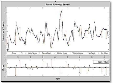
Fig.10. MLPFFNNBP, Best monthly water demand prediction Result

In a more graphic way, we can see the comparison produced by the MLPNNs-LM model between the actual data representing the test data that came from reality and the prediction values according to the model adopted, so figure 11 illustrates this.

When the PB algorithm with LM is used to train MLPNNs it is important to let it is executed until its parameters have converged, which decrease the effect of the initial randomness of the values of the weights. As shown the figures 10, 11, the MLPNNs-LM can predict the next year values with good accuracy as shown in table 2.

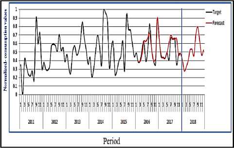
Fig.11. Comparison between reality and the prediction values

• C.    Monthly Prediction RBFNN with the Genetic Algorithm Model

To prediction the water demand in monthly style, we also compute the total consumption as we do the same steps in MLPNNs-LM with the Back Propagation model. Using RBFNN improve and optimize the selection of parameters centers c, radius r . The results of applying the proposed model for data is depicted in figure 12 and table 3 for errors values. Table 3 shows the mean square error values of training and testing incrementally starting from (5) neurons to (60) neurons by increasing (5) neuron in every cycle.

Table 3. RBFNNs -Genetic Algorithm (monthly water demand Prediction Result)

No of Neurons	MSE train	MSE test
5	2.77E-02	1.92E-01
10	2.69E-02	1.30E-01
15	2.10E-02	1.75E-01
20	1.77E-02	1.59E-01
25	1.60E-02	2.20E-01
30	1.54E-02	2.40E-01
35	1.41E-02	2.20E-01
40	1.25E-02	2.30E-01
45	1.30E-02	2.40E-01
50	1.60E-02	2.40E-01
55	1.93E-02	2.50E-01
60	2.59E-02	2.50E-01

According to table 3 and figure 12, it is clear that the RBFNNs with a GAs approach made a weak result for the prediction according to an appropriate quantity of neurons in the hidden layer, thus our prediction mean square error (MSE) on 60 neurons appear low result for the future of monthly water demand with mean square the values of the

MSE during the test period in accepted were it's not very well, this because the pattern of the training process is not ordered during the tested data of the last 7 years. This problem in the patterns will appear in the next applied model which use RBFNNs optimized with GAs.

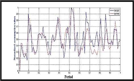
Fig.12. RBFNN-GAs, Best monthly water demands Prediction Result

In a more graphic way, we can see the comparison produced by the RBFNNs-GAs model between the actual data representing the test data that came from reality and the prediction values according to the model adopted, so figure 13 illustrates this.

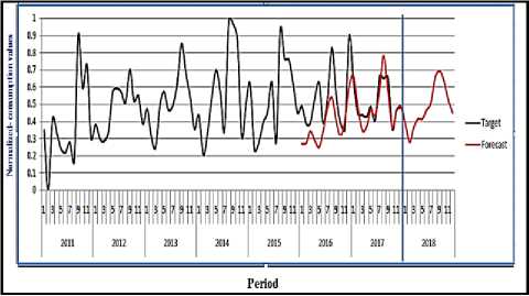
Fig.13. Comparison between reality and the prediction values

• D.    Comparison and Discussion

We made a comparison according to the performance from the perspective of the error value versus the number of neurons employed, in figure 14 the values of errors for MLPNNs-LM and RBFNNs-GAs is represented versus a number of neurons to display the trend of error for predicting.

We can see the excellence of MLPNNs with LM from the first prediction process until the end by employing the increased number of neurons. In the other hand, we can see the less performance for RBFNNs with GAs; hence there is a clear and visible superiority in favor of MLPNNs-LM.

We present a comparison between all results obtained from applied models both the neural network and Stochastic Models in this thesis. The following table offers the best values of mean square error (MSE) that generated by MLPNNs-LM, RBFNNs-GAs and ARIMA training and testing stage that utilized to predict water demand consumption. The selected (ANNs) models and ARIMA has been used in order to predict the municipality of Jenin short-term water consumption. Predictions have been made from the year 2011 until 2017. Table 4 present the results produced by the developed ANNs models add to that the ARIMA model.

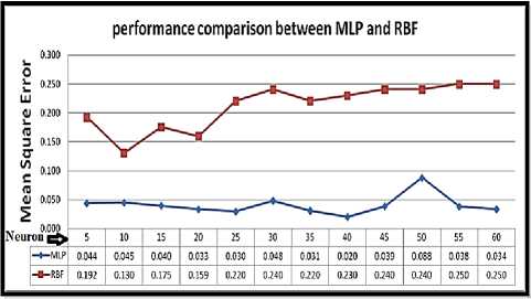
Fig.14. MSE Errors trend of the two neural networks applied models

This experimental result shows the potential of the applied neural networks models especially the MLPNNs with LM in the control in real time of monthly prediction of water demand since they are met during the generalization correlations of 98% and MSE magnitudes of 2%.

Table 4. Mean square error (MSE) Value for Three Model Comparison

Models	No of neurons	MSE train	MSE test
MLPBP with LMA	60	0.0005	0.033
RBF with G.A	60	0.025	0.250
ARIMA	Not support it	0.028	0.051

According to the previous table, we can notice clearly that the prediction result based on (MSE) which generated by the MLPNNs-LM model is preeminent among the other models and it achieves the best result and accuracy, the minimum MSE obtained during the training process of the ARIMA model and RBFNNs-GAs is worse than that in the MLPNNs-LM. Thus, the MLPNNs-LM produced a more accurate output than the RBFNNs-GAs and ARIMA models. The testing showed that the RBF with genetic algorithm in particular generated unsatisfied value even if compared with ARIMA model and ARIMA had resulted not too far away from MLPNNs-LM in water demand simulation but the MLPNNs-LM stayed the best and superb in results.

• VII.    Conclusions

The modeling was based on collected data from all neighborhoods of Jenin city including the consumption as well as these available in the department of water database that follow the municipality. It is clearly observed that in our country there are no applied models that predicted the water demand and consumption or discussed until now. The algorithms were applied to water demand to predict the future of water needs according to the breadth and increase of demand that happen with the time passage. The major interest of this thesis was to assess these algorithms over our datasets, then select and determine the most suitable and accurate one to predict the needs of the coming years.

The applied Neural Networks models have shown a very good prediction of the monthly demand for urban water in the Jenin city. Considering as input variables which present the time data series of the water demands and the objective data is the real water consumption during the time series data. The applied models used to recognize the patterns in the historical data of the water demand, and use this pattern to predict the future data of water demand.

After a number of modeling trials, ANNs particularly is the best model for predicting the water demand and consumption especially the MLPNNs with LM algorithm and achieve a better result than ARIMA and also RBFNNs with GAs. The model produced very good results depending on the high correlation between the actual and predicted values of water demand based on the MLPNNs-LM model. This characterization of short-term demand aims to use as an entry into methods and/or management programs in a real-time of the water distribution system. We plan to search for new sources of information and data is available such as temperature factors, population growth, and other factors in order to link them to prediction processes using the modern artificial networks methodology. Models will be expanded and disseminated in different sectors in cooperation with the Palestinian Water Authority and other applications will be developed in the field of future predictions to improve conditions in our lives and to contribute and to enrich the scientific research fields in our country.