Processing of Satellite Digital Images for Mapping Atmospheric Transmissivity in Bangladesh

Published Online March 2013 in MECS

Atmospheric transmissivity of solar radiation of any region is affected mainly by climatic parameters. Over space and time, the interactions of these climatic controls over different areas cause different temperature and moisture features that affect transmittance property of the atmosphere. Knowledge of atmospheric transmissivity is important in estimating the impact of a polluted atmosphere on weather and climate change and in studying air pollution and energy exchange over polluted regions.

Atmospheric transmissivity can be determined from ground based meteorological data or data from satellites. Some of the methods that use historical weather data for calculating τ are: models based on incoming solar radiation [1-2], model based on sunshine hour [3-4], model based on temperature [5-6], model based on rainfall data [7] etc. And atmospheric transmission factor determined from satellite based model [8].

Kambezidis et al. [9] investigated the diurnal variation of total spectral transmittance of solar irradiance under dominant wind conditions over Athens. The spectral transmittance values estimated were derived using ground-based spectral measurements of beam irradiance in the range 310–575 nm (UV and VIS). The data were recorded by a system consisting of an automatic solar tracker and a spectrometer. All data were recorded under clear-sky conditions in the city center of Athens and the spectral total atmospheric transmittance was estimated towards zenith to avoid optical mass effects.

E. I. Terez and G. A. Terez [2] developed a systematic monitoring method of spectral atmospheric transmission (SAT) in the Crimea (a peninsula in Ukraine) since 1996. A sun-tracking solar photometer that records signals in five spectral regions selected by interference filters centered at 357, 401, 448, 512, and 750 nm, respectively, is used for this purpose. The SAT values obtained during 1996–2000 are compared with the results of earlier studies conducted in the Crimea in 1924–32 (the first observation period) and 1972–90 (the second observation period).

Through the use of the Ångström-Prescott model, Baigorria et al. [10] estimated transmissivity with data from fifteen weather stations from the Peruvian national meteorology and hydrology service (SENAMHI) over Peru. These models were calibrated using 66% of the daily historical record available for each weather station; the rest of the information was used for validation and comparison.

Duk-Jinand Lyzenga [8] presented a new method for estimating the atmospheric transmittance and wind speed over the ocean from WindSat satellite data using a simplified model that uses ocean surface reflectivity.

Yoshihiro Matsuda et al. [7] analyzed meteorological data measured in the Himalaya and the Tibetan Plateau. In this study a favorable correlation between precipitation and atmospheric transmissivity of solar radiation is found in terms of monthly values.

Ahmad and Tiwari [11] estimated the cloudiness/haziness factors and atmospheric transmittances using polynomial regression analysis for the composite climate of New Delhi (latitude: 28.58o N; longitude: 77.02o E; elevation: 216 m above msl). Meteorological data for this study was obtained from Indian Meteorological Department. Atmospheric transmittances for beam and diffuse radiation have been introduced to take into account the uncertain behaviour of atmospheric conditions.

Sun Ji-yin [12] presented a simplified computation algorithm of atmospheric transmittance analyzing data of absorption attenuation of the atmospheric gas such as steam and carbon dioxide.

By using Sambo’s and Chauliget’s model W.E. Alnser and AL-Mudifa[13] was calculated the atmospheric transmission factor for Bahrain. The average atmospheric transmittance was found to be (0.48±.28) in using the former method and (0.76±.007) in the latter one.

The present study investigates the potential of using Advanced Very High Resolution Radiometer (AVHRR) sensor data from National Oceanic and Atmospheric Administration (NOAA) satellite of USA for mapping atmospheric transmissivity of solar radiation using a simple methodology applicable to the tropical environment.

The remainder of this paper is organized as follows: Section 2 gives an effective method of preprocessing satellite images and step by step procedure of determining atmospheric transmissivity. Section 3 describes the seasonal and yearly variation of atmospheric transmissivity over the surface area of Bangladesh. Discussions on the results are also included in this section. Conclusion is given in the final section.

• II.    Methodology2.1    Processing of Satellite Images

• 2.1.1    Satellite image acquisition

• 2.1.2    Noise removal

Meteorological satellites such as NOAA, GOES, METEOSAT, INSAT etc. provide images of brightness over large areas of the earth’s surface. These brightness values can be converted to incoming solar radiation at ground to observe microclimate characteristics. The following sections provide step by step description of the developmental stages of satellite based methodology using NOAA-AVHRR images.

The National Aeronautical and Space Administration (NASA) and National Oceanic and Atmospheric Administration (NOAA) operated Polar Operational Environmental Satellite (POES) offers an alternative to surface measurements. In this study digital data of Advanced Very High Resolution Radiometer (AVHRR/3) from sun synchronous NOAA satellites are used. The characteristics of NOAA images are given in Table 1.

Table 1: Characteristics of NOAA- AVHRR Images

Satellite Name	Sensor	Satellite ID	Spatial Resolution	Radiometric Resolution	Sensor View Angle
NOAA-KLM Series	AVHRR/3	NOAA-15, 16 and 17	1.1×1.1 km at nadir	16 bit	55 deg

The space-borne AVHRR/3 radiometer data are downloaded by the 1.2m, L-band satellite antenna. The antenna system is a continuous time tracking and sensitive at the frequency of 1695 - 1710 MHz.

Communication between satellite and ground station is happened by the high resolution picture transmission (HRPT) mode. In Bangladesh, the data of NOAA satellite is captured by the ground receiving station situated at Bangladesh Space Research and Remote Sensing Organization (SPARRSO) in Dhaka. The images are generated by Kongsberg Spacetec S,A, Ltd. Multimission Earth Observation System (MEOS). Radiometric resolution of the image data is of 16 bit. Images of one complete year (February 2005 to January 2006) from NOAA-17 are taken for this study.

Image noise is any unwanted disturbance in image data that is due to limitations in the sensing, signal digitization or data recording process [14]. Different sources of this noise could be due to periodic drift or malfunction of the detector, electronic interference among sensor components, or problem in the transmission and recording process. The noise, if present in any part of the image can either degrade or totally mask the true radiometric information contained by the digital image. Hence, noise removal is very essential before any preprocessing or analysis of the image could be done.

• 2.1.3    Geometric correction and image to image registration of satellite images

  The orbiting satellites, like NOAA, provide images having swath width of about 2399 km. Due to such large swath width, during the scanning process, a number of geometric distortions are introduced into the image data. Also, raw images obtained from the ground receiving stations are not maps. They cannot be used to

find positional parameter of any point on the image or for image to image comparison. Therefore, geometric correction of the images is necessary for achieving required locational accuracy and registering the images with a common map coordinate system.

Geometric correction method

Removing geometric distortion is an important part of image processing. Also this is the most time consuming part of processing. Different geometric correction methods are available. These methods varies from simple scale change and rotation, to non-linear wrapping based on sensor platform and earth dynamics modeling.

In this study, a two-stage process has been applied for the correction of geometric distortions from the images. A pre-rectified reference image is used to register the corrected images with reference to this image. In the first stage, an empty matrix in the map coordinate systems is created. Then the transformation of old coordinates to new coordinates is carried out through an affine (first order) or higher order transformation equations of the form:

1st order or affine transformation equation:

X´ = ao + a1x + a2y and

• Y´ = bo + b ₁ x + b ₂ y                            (1)

2nd order transformation equation:

X´ = ao + a1x + a2y + a3x2 + a4y2 + a5xy and

• Y´ = b o + b 1 x + b 2 y + b 3 x² + b 4 y² + b 5 xy           (2)

• 2.1.4    Radiometric calibration and conversion of DN values to physical parameters

where X´ and Y´ are coordinates for image and x and y are for map. The coefficients ao-a5 and b0-b5 are determined by minimizing the sum of squared errors using least squares technique.

Table 2: Geocorrection and projection parameters adopted in this study

Transformation type	Polynomial
Transformation order	Second order
Map projection	Lambert conformal conic (LCC)
Resampling method	Nearest neighbor

In the second stage, a suitable resampling method is employed to assign DN values to the output matrix pixels. The rectified images are intended to use for solar radiation estimation. In the rectification process, therefore, minimum changes in the original DN values are expected. To satisfy this condition, we have used nearest neighbor interpolation method for resampling- as this method (nearest neighbor) transfers the original pixel brightness values without averaging them. Image processing has been done using ERDAS IMAGINE® software. In the geometric correction process, distortions of the navigated images are corrected by using ground control points selected manually. About 20 GCPs are used for each image. Table 2 shows the geocorrection and projection parameters adopted in this study. In our case the image size is large (about 1024 x 1024 pixels) which contains different surface terrain, so the 2nd order transformation equation has been used for achieving required accuracy.

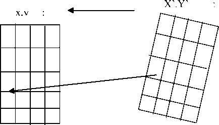
Fig. 1: Transformation from one coordinate system to another

Radiometric calibration of the AVHRR visible and near-infrared channels (channel 1 and 2) is an important consideration. Although NOAA performs pre-launch calibration, it is not sufficient to relay on these calibration data alone to achieve the desired accuracy from AVHRR data (NOAA data user’s guide, section-3). The instrument characteristics cannot be expected to remain the same in orbit as they were before launch. This situation occurs primarily because the thermal environment varies with the satellite’s position in orbit, causing the output in digital counts to vary. Initially, Channel 1 and 2 are observed to degrade in orbit because of the launch associated contamination. Continued exposure to the harsh space environment is also a contributing factor [15]. In addition, the performance is degraded with the instrument’s components age in the years that elapse between the pre-launch tests and the years that the instrument is typically operational. Using these coefficients, raw digital counts can be converted to the corrected top of atmosphere (TOA) reflectance using the formula (NOAA Data User’s Guide)

Ref i (l,c) = S i × DN i (l,c) + I i                         (3)

where, Ref = percent reflectance; i = channel number 1, 2 or 3A; l,c = image coordinate (line and column number); Si = slope (gain) for band i;

Ii = intercept for band i; and DNi(l,c) = digital count value for band i at pixel (l,c).

• 2.1.5    Sun angle effect and sun-earth distance effect correction

Besides radiometric changes, there is solar illumination variability along the orbital path (north/south direction). Solar illumination changes in the north/south direction with an orbit are corrected using the cosine of solar zenith angle as:

Corrected reflectance =

Original reflectance × (d²/cosθ)         (4)

where, d2 = eccentricity correction factor and

• θ = solar zenith angle.

• 2.2    Determination of incident solar radiation using satellite data

• 2.2.1    Cloud Cover Index

Here d is the sun-earth distance expressed in astronomical units and d2 generally referred to as the earth-sun distance correction factor, accounts for the seasonal variations in the solar irradiation at the top of the atmosphere.

Incident solar radiation map for the whole country was constructed using a satellite based statistical model which was developed in our previous study [16-17]. Detail description of the method is out of the scope of this paper. For sake of clarity a brief description is given here. The methodology employed in this work is a statistical approach. The basic idea of the model is that the amount of cloud covering over a given area statistically determines the global solar radiation received by that area. The first step of the methodology is the determination of cloud index for each point on the image (i,j), called a pixel. The second step is to find the total atmospheric transmission factor from the ground measured values. The third step is to find the model coefficients from a linear relation of cloud index and atmospheric transmission factor which is then used in the final step for the estimation of global solar radiation using the model.

Cloud cover index, nt(i,j), for a particular pixel (i,j) at a time t, can be defined as [18-19]

nt

rapp (i, j ) - rclear (i, j ) rcloud (i, j ) - rclear (i, j )

where rapp(i,j) is the instantaneous/apparent planetary reflectance sensed by the satellite radiometer; rclear(i,j) is the clear sky planetary albedo corresponding to a reflectance for the clear sky earth’s surface plus the dry atmosphere above it and rcloud(i,j) is the reflectance for the overcast cloud including albedo of cloud top and atmosphere above the cloud.

• 2.2.2    Finding model coefficients

• 2.2.3    Estimation of solar radiation

• 2.2.4    Determination of atmospheric transmissivity

For running the model, first we need some training data. These data are obtained from some test ground stations that measure incoming solar radiation. These incoming solar radiation data along with the satellite data are used to find model coefficients (or regression coefficients). For short durations (for a month), these coefficients were considered constant.

Once regression coefficients of an area are known, they are used to estimate hourly global solar radiation for that area. Solar radiation maps for the whole country are obtained through extrapolation. Monthly solar radiation maps are derived from the daily hourly maps.

Atmospheric transmissivity or atmospheric transmission coefficient, or clearness index, τ, is the ratio of global solar radiation at ground level to extra terrestrial solar radiation. The transmissivity was calculated in this paper using

T = I s /I o                                       (6)

where Is (kJ m-2 h-1) is the solar radiation incident on the earth surface at a certain point averaged over an hour and I0 (kJ m-2 h-1) is the hourly extraterrestrial solar radiation over a horizontal surface at the same point.

I0 was calculated using the following equation [20]

I 0 = I x E 0 (sinδ sinφ +

(24 /π ) sin(π / 24) cosδ cosφ cosω_i )         (7)

where I is the solar constant, E ₀ is the eccentricity correction factor, δ is solar declination, φ is the latitude and ωi is the hour angle at the middle of the hour. Is was determined through processing of satellite images as described in section 2.2. The obtained monthly average incident radiation map was divided into latitude and longitude grids and radiation values on surface level and extraterrestrial radiation for each intersecting grid points were recorded. Transmissivity values for the grid points were then calculated using (4). Values of τ for the grid points were taken as input to SURFER^® software to construct map of τ for the whole study area. Spatio-temporal distribution of τ was studied by preparing monthly maps for the whole country for twelve months (February 2005 to January 2006). Yearly average map was prepared by integrating the monthly average maps. Overall procedure for mapping atmospheric transmissivity has been shown in Fig 2. Processing of satellite images was done using Erdas Imagine® software.

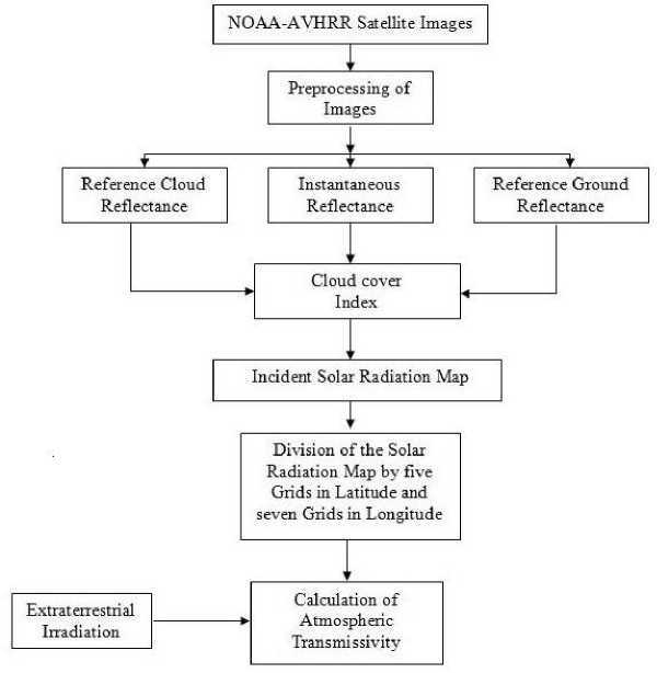
Fig. 2: Flow diagram for finding atmospheric transmissivity from satellite images

• III.    Result and Discussion

In this work, we have estimated the spatial distribution of atmospheric transmissivity of solar radiation for wavelength band 0.3μm to 3.0μm using NOAA-AVHRR satellite data. Following figures (Figure 3 and Figure 4) show the results for the study period. The values presented here are monthly average hourly values for the hour 10:00 am to 11:00 am LST (local standard time) which is designated as 10:30am.

Fig 3(a) and 3(b) show the spatial variation of atmospheric transmissivity for the months of January and February. Transmissivity values in these months were observed to increase progressively from southern region to northern region. For these months transmissivity value for the country was seen to vary from 0.43 to 0.59.

Fig 3(c) shows monthly variation of average transmissivity over the country for March. For this month transmissivity value varies in the reverse direction as that was seen in the previous month. Northeastern parts of the country were seen to have lower transmissivity values whereas southern parts have higher values.

Fig 3(d), 3(e) and 3(f) show map of τ for April, May and June respectively. Relatively higher value of transmissivity (0.45 to 0.64) was observed all over the country for these summer months. Fig 3(g), 3(h), 3(i) and 3(j) show the spatial variation of τ for the months of July, August and September. From July, transmissivity value was seen to decrease sharply from that was observed in June. For these months transmissivity value was between 0.34 and 0.50. In June, the atmosphere of the western zone of the country was seen to be more transparent than that in the eastern zone. For other months except some local variability, transmissivity values were more or less same over the country.

Fig 3(k) and 3(l) show the spatial variation of transmission factor for the months of November and December. In November the lowest value of transmissivity of the year was recorded for the country (0.35 to 0.44). In December, a little increase of τ was observed. It was noticed from the figures that in November transmissivity value increased from northern to southern direction whereas in December this value increased from southern to northern direction.

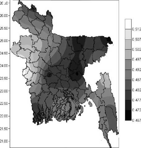
Fig 4 shows the yearly average map of transmissivity over the land surface area of Bangladesh. Yearly average map shows that there is a small spatial variation of transmissivity over the country. Transmissivity value varies from 0.467 to 0.512. The higher transmittance areas are the mid-western and north-western parts and in eastern hilly areas.

Bangladesh is primarily a low-lying plain situated on deltas of large rivers flowing from the Himalayas. Geographically, it extends from 20˚34´ N to 26˚38´ N latitude and from 88˚01´ E to 92˚41´ E longitude. Bangladesh has a sub-tropical humid climate characterized by wide seasonal variations in rainfall, moderately warm temperatures and high humidity [21].

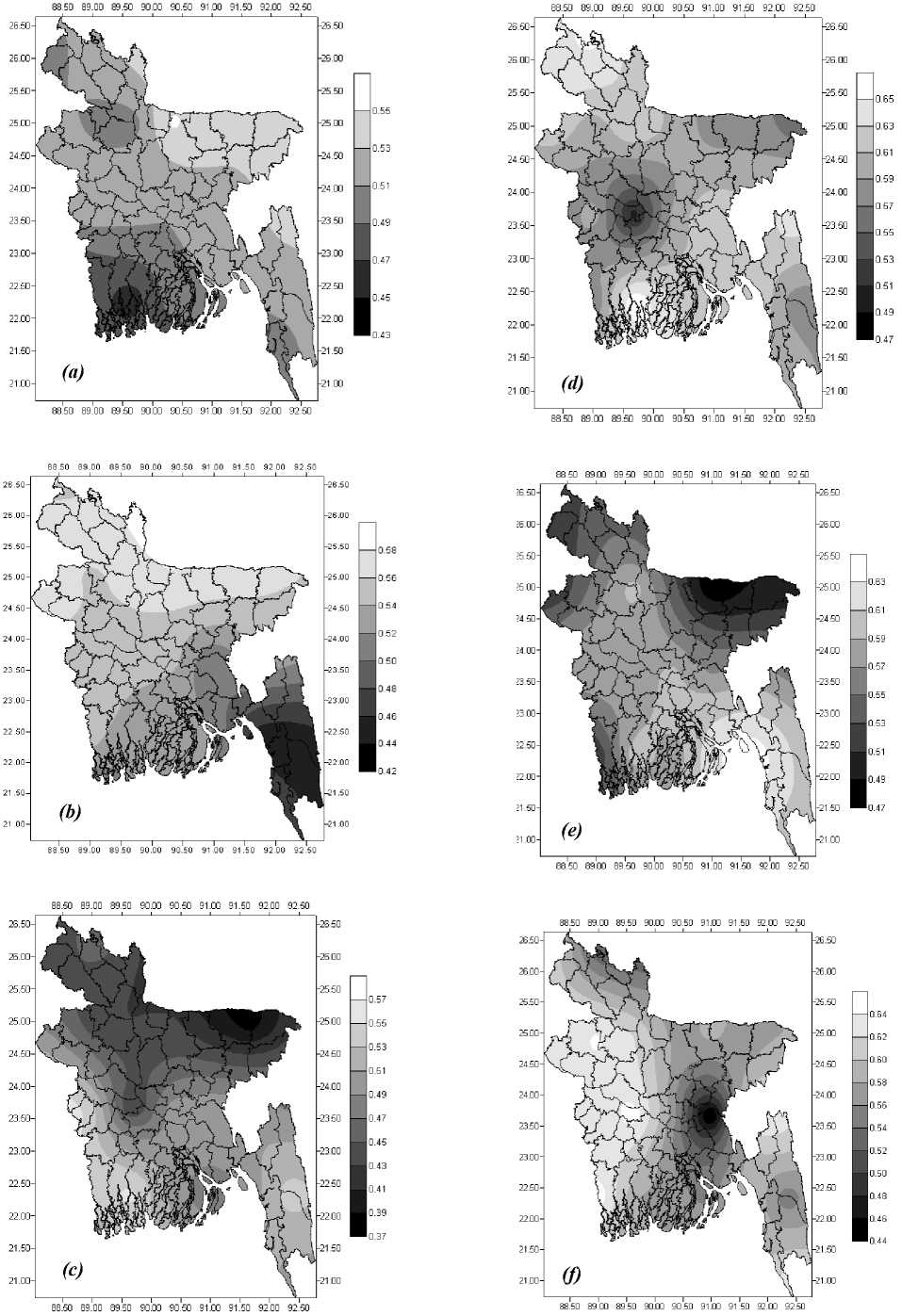
Fig. 3: Monthly average transmissivity map of Bangladesh for (a) January (b) February (c) March (d) April and (e) May and (f) June at 10:30 am.

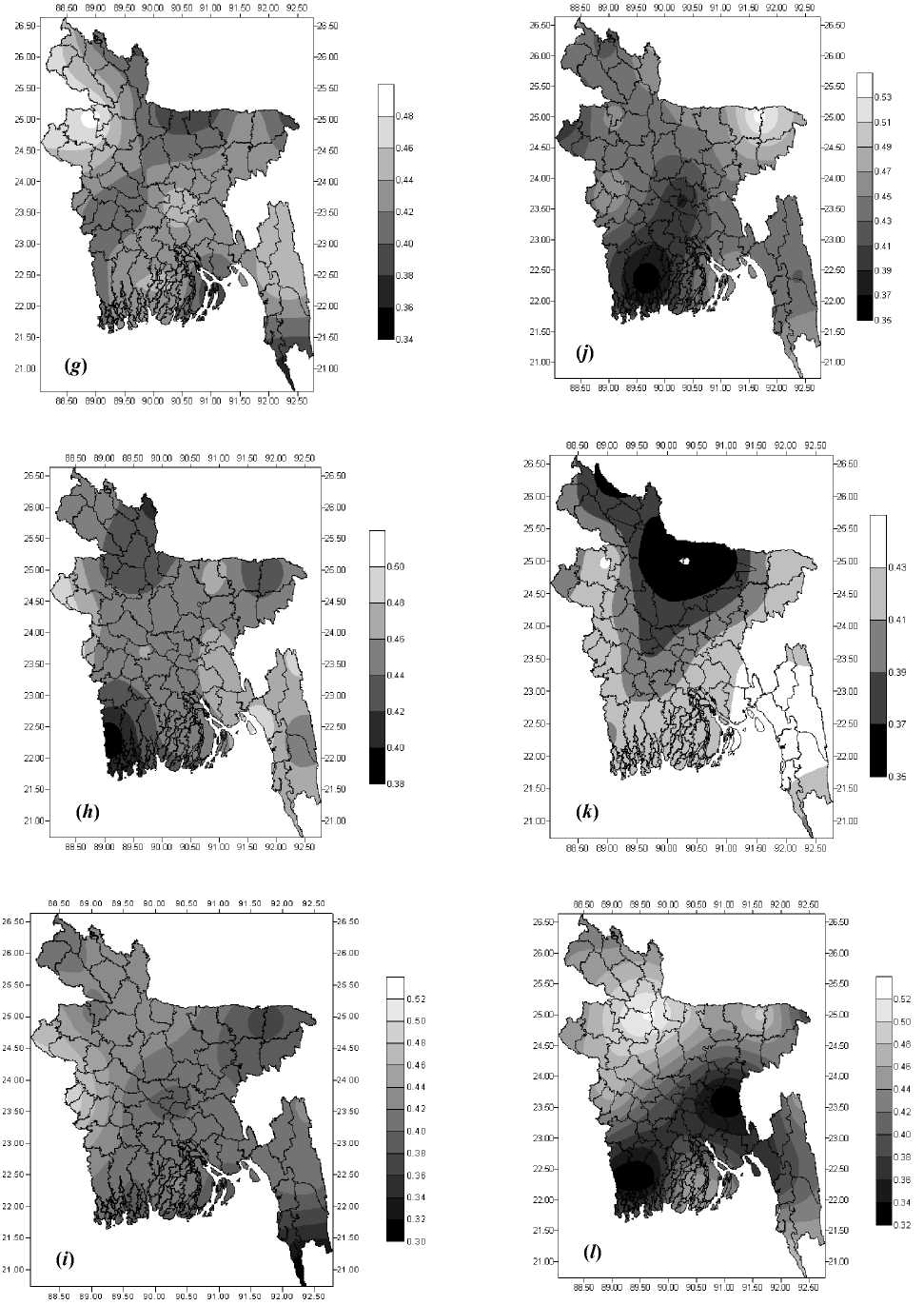
Fig. 3 continu: Monthly average transmissivity of Bangladesh for (g) July (h) August (i) September (j) October (k) November and (l) December at 10:30 am.

Four distinct seasons can be recognized in Bangladesh from the climatic point of view: (1) the dry winter season from December to February, (2) the premonsoon hot summer season from March to May, (3) the rainy monsoon season from June to September and (4) the post-monsoon autumn season which lasts from October to November. Rainfall variability in space and time is one of the most relevant characteristics of the climate of Bangladesh. Rainfall in Bangladesh varies from 1400 mm in the west to more than 4300 mm in the east of the country [22].

88.50 39.00 8950 90.00 90.50 91.00 91.50 ЦЙЗ.ОО' 196.50

Fig. 4: Yearly average map of atmospheric transmissivity over Bangladesh

The map sequence (Fig 3(a) to 3(l)) clearly shows the seasonal variation of τ, with maximum values in the summer months of April to June and minimum values in November.

From January to March, high solar radiation areas expand progressively from south to north. This is mainly due to the change of sun’s declination toward the celestial equator, causing an increase of latitude. Cloudiness plays a less important role in this increase because in this period skies in most parts of the country remain relatively clear. The irregular transmissivity distribution patterns in some areas and for some times may due to local climatic conditions.

During the pre-monsoon season (March to June), climate of Bangladesh is characterized by high incident radiation, high temperatures and sometimes occurrence of thunderstorms. Thunderstorms are the sources of premonsoon rainfall of Bangladesh [23]. Thunderstorms are the small scale local activity that affects transmissivity locally. As a result, lower transmissivity values may be observed in some areas of western and northern regions of the country. In April, the Sun’s declination is near the celestial equator, as a result higher radiation is incident all over the country. In addition, it is in a period of the dry season skies for most parts of the country are still relatively clear with low cloud frequency. This may be the cause of observing highest level of transmissivity.

Although, during July to September, extraterrestrial radiation is on the higher level for the whole country, effect of the southwest monsoon, in terms of rainfall and cloudiness, is strongly dominated. In this southwest monsoon period the precipitation is one order of magnitude more than during the rest of the year [24]. Consequently, the transmissivity of atmosphere is reduced in the rainy periods than that of summer months.

From September to December, apparent sun’s path in the sky moves southward from the celestial equator, resulting in a slanting path for beam radiation from the Sun. As a result transmittance values remain relatively lower. In October, the winter monsoon begins that brings dry and cool air all over the country, causing clearer skies. During winter periods sun’s radiation has to travel through long air causing lower transmissivity for the whole country. Lowest level of τ can be observed at some places may due to the persistence of fog and other anthropogenic activities.

• IV.    Conclusion

A simple method has been developed through the processing of NOAA- AVHRR satellite images to find the atmospheric transmissivity for Bangladesh. Data of twelve months have been processed to observe the spatio-temporal variation of τ over surface area of Bangladesh. It is observed that the geographical distribution of τ exhibits patterns and trends. No prior study has been done on the transmittance property of atmosphere on Bangladesh. Therefore it is not possible to make any comparative study or make any comment on the results.

Acknowledgement

Data of remote sensing satellites are obtained from Bangladesh Space Research and Remote Sensing Organization (SPARRSO), Dhaka.