Protection of Thyristor Controlled Series Compensated Transmission Lines using Support Vector Machine

Author: A.Y. Abdelaziz, Amr M. Ibrahim
Journal: International Journal of Intelligent Systems and Applications(IJISA) @ijisa
Article in issue: 5 vol.5, 2013.
Free access
Recently, series compensation is widely used in transmission. However, this creates several problems to conventional protection approaches. This paper presents overcurrent and distance protection schemes, for fault classification in transmission lines with thyristor controlled series capacitor (TCSC) using support vector machine (SVM). The fault classification task is divided into four separate subtasks (SVMa, SVMb, SVMc and SVMg), where the state of each phase and ground is determined by an individual SVM. The polynomial kernel SVM is designed to provide the optimal classification conditions. Wide variations of load angle, fault inception angle, fault resistance and fault location have been carried out with different types of faults using PSCAD/EMTDC program. Backward faults have also been included in the data sets. The proposed technique is tested and the results verify its fastness, accuracy and robustness.
Fault Classification, Fault Detection, Overcurrent Protection, Distance Protection, Thyristor Controlled Series Compensated Transmission Line, Support Vector Machine
Short address: https://sciup.org/15010416
IDR: 15010416
Text of the scientific article Protection of Thyristor Controlled Series Compensated Transmission Lines using Support Vector Machine
Published Online April 2013 in MECS
The use of FACTS devices to improve the power transfer capability in high voltage transmission line is of greater interest in these days. The thyristor controlled series compensator (TCSC) is one of the main FACTS devices, which has the ability to improve the utilization of the existing transmission system. TCSC based compensation possess thyristor controlled variable capacitor protected by Metal Oxide Varistor (MOV) and an air gap. However, the implementation of this technology changes the apparent line impedance, which is controlled by the firing angle of thyristors, and is accentuated by other factors including the metal oxide varistor (MOV). The presence of the TCSC in fault loop not only affects the steady state components but also the transient components.
The controllable reactance, the MOVs protecting the capacitors and the air-gaps operation make the protection decision more complex and, therefore, conventional relaying scheme based on fixed settings has its limitation. Fault classification is a very challenging task for a transmission line with TCSC. Different attempts have been made for fault classification using Wavelet Transform [1], Kalman filtering approach [2] and neural network [3].
The Kalman filtering approach [2] finds its limitation, as fault resistance cannot be modeled and further it requires a number of different filters to accomplish the task. BPNN (back propagation Neural Network), RBFNN [4] (radial basis function neural network), FNN (Fuzzy Neural network) are employed for adaptive protection of such a line where the protection philosophy is viewed as a pattern classification problem [5]. Furthermore, combined techniques have already been used, such as wavelet transform and fuzzy logic [6, 7]; neural network and fuzzy logic [8, 9]; neural network and wavelet transform [10].and neural network and total least square estimation of signal parameters via the rotational invariance [11]. The networks generate the trip or block signals using a data window of voltages and currents at the relaying point. However, the above approaches are sensitive to system frequency changes, and require large training sets and training time and a large number of neurons.
The paper presents an approach for fault classification of TCSC based line using support vector machine (SVM). SVM, basically, is a classifier based on optimization technique. It optimizes the classification boundary between two classes very close to each other and thereby classifies the data sets even very close to each other. Also SVM works successfully for multiclass classification with SVM regression.
The current or current and voltage signals for all phases are retrieved at the relaying end at a sampling frequency of 1.0 kHz. The inputs to SVMs are post fault current samples or current and voltage samples (half cycle data (10 samples)). Also samples for healthy system are taken as inputs to SVMs. Two SVM are used SVMabc and SVMg. both SVMs are trained with all the ten types of possible short circuit faults (e.g., a-g, b-g, c-g, a-b, b-c, c-a, a-b-g, b-c-g, c-a-g, a-b-c-g) in addition to normal state. The SVM is trained with input and output sets to provide most optimized boundary for classification. This issue is taken care by SVMs as the total half cycle (10 samples) data of the fault current or current and voltage signal(s) is taken into consideration for training and testing the SVMs. The paper is organized as follows. Section II gives a description of power system with thyristor controlled series capacitor (TCSC). Section III presents an introduction of Support Vector Machine (SVM). Sections IV discus the results of using SVM on the protection of the system under study with changing system parameters such as fault location, fault type, fault inception angle and fault resistance. Finally, the conclusion of this study is presented in Section V.
-
II. Power System under Study
A study system is constructed utilizing the EMTDC/PSCAD package [12]. The series-compensated EHV transmission line modeled in this simulation is based on a three phase 230 kV line. The system has two equivalent sources; the TCSC is located close to the midpoint of the transmission line. Two fixed series capacitors are connected in series with the TCSC. The over-voltage protection of the TCSC is provided by the MOV and the protective firing of the thyristors. The over-voltage protection of the fixed capacitors (Cf1 = 48 microfarad and Cf2 = 66 microfarad) is also provided by MOVs. The transmission line model used in the simulation is the distributed parameters model.
The TCSC control will bypass the series capacitor (Cf3 = 177 microfarad) during fault by fully gating the thyristors. The power system frequency of 50 Hz was used. The loading conditions are represented by ten degree load angle. The volt-ampere characteristics of the MOV protection are calculated as in [13].
The characteristics of the source impedance:
+ ve Sequence:
R = 2 ohm
X L = 200 ohm
Zero Sequence:
R = 0.2 ohm
X L = 20 ohm
The characteristics of line # 1 and line # 2:
+ ve Sequence:
R = 1.31 e-4 ohms/m
X L = 6.7038 e-4 ohms/m
X C = 176.8388 Mohms*m
Zero Sequence:
R = 0.262 e-3 ohms/m
X L = 1.34042 e-3 ohms/m
X C = 318.30984 Mohms*m
The system is completely transposed and has communication channels between phases. A single line diagram of the study system is shown in Fig. 1.
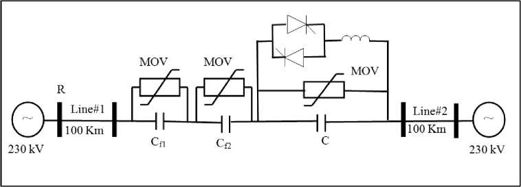
Fig. 1: System under study
A distributed parameters model is used for transmission lines. The TCSC control is assumed to bypass the series capacitor during faults by fully gating the thyristors. Different fault locations and fault types are simulated to test the relay performance. Voltage and current signals seen by the relay at R are obtained at the line terminals. Simulations are performed using an electromagnetic transient program, EMTDC/PSCAD. Sampling frequency is 1.0 kHz at 50 Hz base frequency. The generated waveforms are represented. Fig. 2 through Fig. 5 shows waveforms of the fault voltage and current signals for different fault types. For example, at 30 % and 70 % fault locations.
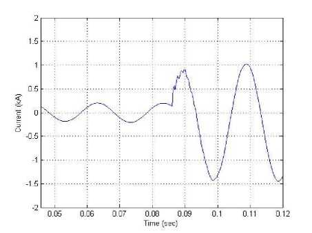
Fig. 2: Phase "A" Current (kA), for line to ground fault “A-G” at 30 % of line
"2‘ 0.05 CLOS 0.07 CLOS 0.09 0.11 0J2
Time (sec)
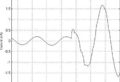
Fig. 3: Phase "A" current (kA), for line to line to ground fault “A-B-G” at 70 % of line
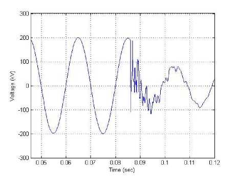
Fig. 4: Phase "A" Voltage (kV), for line to ground fault “A-B” at 30 % of line
It is a computational learning method based on the statistical learning theory. While traditional statistical theory keeps to empirical risk minimization (ERM), SVM satisfies structural risk minimization (SRM) based on statistical learning theory (SLT), whose decision rule could still obtain small error to independent test sampling. SVM mainly has two classes of applications, classification and regression. In this paper, application of classification is discussed.
The classification problem can be restricted to consideration of the two-class problem without loss of generality. In this problem, the goal is to separate the two classes by a function (a classifier), which is induced from available examples and work well on unseen examples, i.e. it generalizes well.
There are many possible linear classifiers that can separate the data, but there is only one that maximizes the margin (maximizes the distance between it and the nearest data point of each class).
This linear classifier is termed the optimal separating hyperplane. Intuitively, this boundary could be expected to generalize well as opposed to the other possible boundaries.
Given a set of training data
{xi,У J, i =1
,...,
n, y. e - 1,1}, x. e Rd
, i , , i (1)
Each x i is a d-dimensional real vector R d . The points x which lie on the hyperplane satisfy:
w . x + b = 0
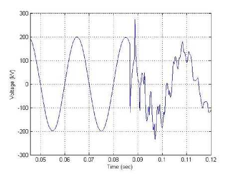
Fig. 5: Phase "A" Voltage (kV), for line to line to ground fault “A-B-G” at 70% of line
-
III. Support Vector Machine
Support vector machine [14-16] was originally introduced by Vapnik and co-workers in the late 1990s.
Where w is normal to the hyperplane, |b|/||w|| is the perpendicular distance from the hyperplane to the origin, and ||w|| is the Euclidean norm of w. For the linearly separable case, the support vector algorithm simply looks for the separating hyperplane with largest margin. This can be formulated as follows (suppose that all the training data satisfy the following constraints):
x; . w + b >+ 1 for yt =+ 1
x;. w + b <— 1 for yt =—1
These can be combined into one set of inequalities:
yi(xi. w + b) — 1 > 0 , for all i
Now consider the points for which the equality in (3) holds. These points lie on the hyperplane H1: xi. w + b = 1 with normal w and perpendicular distance from the origin |1-b|/||w||. Similarly, the points for which the equality in (4) holds lie on the hyperplane H2: xi. w + b = -1, with normal again w, and perpendicular distance from the origin |-1-b|/||w||. It is noticed that H1 and H2 are parallel and the margin is simply 2/||w|| which is observed in Fig. 6. Training points for which the equality in (5) holds are called support vectors. The pair of hyperplanes which gives the maximum margin by minimizing ||w||, subject to constraints can be found. The optimization problem presented is difficult to solve because it depends on ||w|| which involves a square root. Fortunately it is possible to alter the equation by substituting ||w|| with 0.5||w||2 without changing the solution. Taking into account the noise with slack variable ξ and error penalty C, the optimal hyperplane can be found by solving the following convex quadratic programming (QP) problem:
Minimize
n
-iiW ||2 +с X5 2 i =1
Subject to
У, (xw + b ) > 1 - 5 , 5> 0, fori = 1,..., n (6)
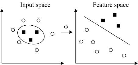
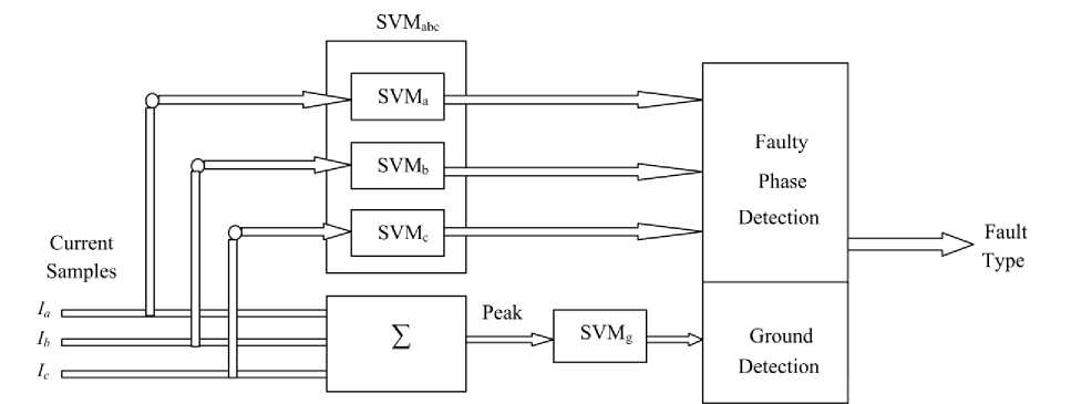
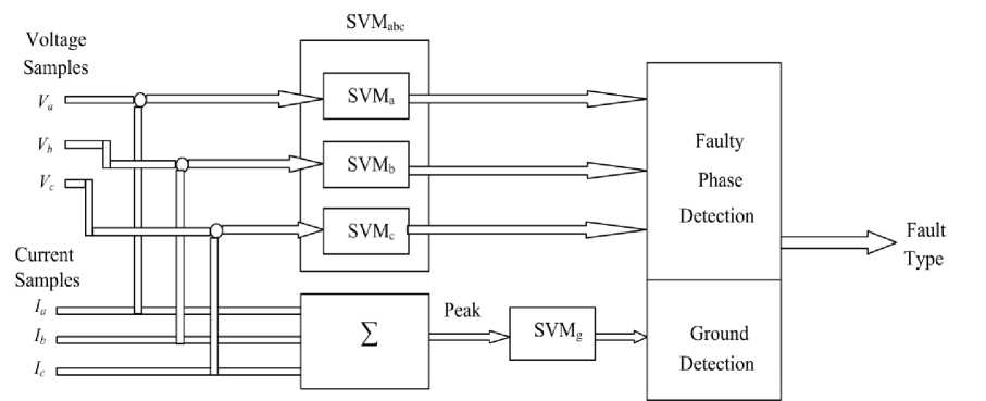
Xya = 0, 0 < a ... ,n If αi > 0, then the corresponding xi is called a support vector. In general, support vectors are only a small part of the training samples. Finally, the optimal separating hyperplane is obtained as follows: Va y iX,. x, + b = 0 iii j SVs where SVs stands for Support Vectors. Then the nonlinear classifier decision function is: ,f(x) = sgn Xa-yi-xi+ b V SVs The test data example “x” is classified as follows: Fig. 6: Maximum margin hyper-plane and margins for a SVM trained with samples from two classes x e < Class -1, Class - 2, if f (x) > 0if f (x) < 0 The original optimal hyper-plane algorithm proposed by Vladimir Vapnik was a linear classifier. However, in 1992, Bernhard Boser, Isabelle Guyon and Vapnik suggested a way to create non-linear classifiers by applying the kernel trick to maximum-margin hyperplanes. The resulting algorithm is formally similar, except that every dot product is replaced by a non-linear kernel function. k (x,x') = ф(x ), ф(x')) where ξi is measuring the degree of misclassification, the constant C > 0 determines the trade-off between margin maximization and training error minimization and n is the number of samples. In the present case, it will turn out that it is more convenient to deal with the dual. This can be done by converting the problem with the Karush-Kuhn-Tucker (KKT) conditions into Lagrange optimization dual problem: Maximize This allows the algorithm to fit the maximum-margin hyperplane in the transformed feature space. The transformation may be non-linear and the transformed space high dimensional; thus though the classifier is a hyper-plane in the high-dimensional feature space, it may be non-linear in the original input space Fig. 7. Fig. 7: Mapping the training data into a higher-dimensional feature space nn w (a) = Xa -- X aiajy iV jx i • xj i =1 2 i, j =1 Subject to In this work, the polynomial kernel function with different degrees is used: k (x,x ‘) = (xx,x where n is the polynomial degree. IV. SVMs Training and Testing Four independent SVMs are used for fault classification and ground detection as shown in Fig. 8. SVMa, SVMb and SVMc are used for detection of the fault for phase a, b and c respectively. The fourth SVM, SVMg, is used for ground detection. Training a SVM involves solving a constrained quadratic programming problem, which requires large memory and enormous amounts of training time for large scale problems. In contrast, the SVM decision function is fully determined by a small subset of the training data, called support vectors. Therefore, it is desirable to remove from the training and test sets the data that is irrelevant to the final decision function [16]. In the proposed technique the margin data sets are used for SVM training and test. Using margin data in SVM training and test makes the decision on the proposed method more accurate and efficient. (a) (b) Fig. 8: The proposed protection scheme using (a) current samples or (b) current and voltage samples 4.1 SVMs for Fault Classification: Half cycle current or current and voltage samples after the inception of the fault are used as inputs to SVMabc. The corresponding output is either a fault or no fault. The input current samples and the corresponding output are termed as “x” and “y” respectively. “y” results in “1” for fault and “-1” for no fault and backward faults. SVMs training require selection of the error penalty “C” and kernel function “φ” parameters, which influence the ensuring model performance. A polynomial kernel with different degrees “n” is used for this work. The range of “C” chosen for training is from 10-9to 109and “n” values used are 4 and 6. SVMs is trained with 524 data sets and tested with 162 data sets for all the 10 types of faults and normal conditions. Different error penalty “C” values are used to get the most optimized value for the classification problem and a comparison between different kernel polynomial degrees has been made. The maximum correct predictions percentage for different types of faults with the corresponding error penalty for using current and voltage/current samples are shown in Table 1 and Table 2 respectively. It is noticed that same kernel polynomial degrees are used with different error penalties “C” for current samples inputs and current/voltage samples inputs. The used kernel polynomial degrees are 4 and 6 for both cases. The used values of error penalty are chosen to control the percent of correct predictions and to get the most optimized value for the classification problem. Table 1: Summary of Maximum Correct Predictions Percentage for Current Samples Fault type Kernel polyno--mial degree Error penalty “C” No. of test cases No. of correct predictions Correct predictions, % LG 4 50×104 81 78 96.30 6 45×104 81 79 97.53 LLG 4 3×10⁵ 162 160 98.77 6 4×10⁴ 162 159 98.15 LL 4 6.5×10⁴ 162 158 97.53 6 4.5×10⁴ 162 158 97.53 LLL 4 -- 81 81 100.000 6 -- 81 81 100.000 4 Total 486 477 98.15 6 486 477 98.15 Table 2: Summary of Maximum Correct Predictions Percentage for Current and Voltage Samples Fault type Kernel polynomial degree Error penalty “C” No. of test cases No. of correct predictions Correct predictions, % LG 4 56×105 81 79 97.53 6 36×105 81 79 97.53 LLG 4 2×10⁶ 162 160 98.77 6 3×10⁵ 162 161 99.38 LL 4 1.5×10⁵ 162 159 98.15 6 3.5×10⁵ 162 160 98.77 LLL 4 -- 81 81 100.000 6 -- 81 81 100.000 4 Total 486 479 98.56 6 486 481 98.79 4.2 SVM for Ground Detection: SVMg is trained with the ground current as input “x”. Ground current is resulted from the summation of the three line currents Ia, Ib and Ic. The corresponding output “y” is “1” for the fault involving ground and “-1” for fault without ground. As the ground current is pronounced in case of a fault involving the ground compared to a fault without involving ground, the SVMg is trained to design an optimized classifier for ground detection. SVM is trained with data sets result from summation of Ia, Ib and Ic of fault classification data. Different 162 data sets are used for testing SVM. The accuracy is 100% for kernel polynomial degrees used (2 and 3) and error penalties from C = 10 -9to C = 10 9. V. Conclusion This paper proposes two schemes, overcurrent and distance protection schemes, for fault classification in transmission lines with thyristor controlled series capacitor (TCSC), using Support Vector Machine (SVM). Half cycle post fault samples (ten samples) are used as input to the SVMs and the output is the corresponding classification. The fault classification task is divided into four separate subtasks (SVMa, SVMb, SVMc and SVMg), where the state of each phase and ground is determined by an individual SVM. The three SVMs (SVMa, SVMb, and SVMc) are combined together to a single SVM, SVMabc. The first scheme, overcurrent protection, uses current signals from the inception of the fault as inputs to SVMs. The second scheme, distance protection, uses both voltage and current signals as inputs to SVMs. Both schemes use the ground current (Ia + Ib + Ic) as input to SVMg for ground detection, where Ia, Ib and Ic are currents of the respective phases. Influence of changing system parameters such as fault location, fault type, fault inception angle, fault resistance and pre-fault power flow value has been studied. The algorithm has also been tested for backward faults. The error found is less than 4% for overcurrent protection and less than 3% for distance protection taking all SVMs to consideration. Test results show that the proposed technique is reliable in classifying faults, using voltage and current measurements or current measurements only at one end. The proposed method converges fast with fewer numbers of training samples. The results of the proposed technique indicate the accuracy and the effectiveness of the method. The proposed SVM based technique can be considered to be superior to the other techniques due to good generalization performance, computational efficiency and robust in high dimensions.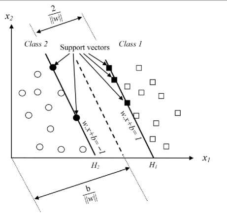
References Protection of Thyristor Controlled Series Compensated Transmission Lines using Support Vector Machine
- P. K. Dash, S. R. Samantaray, “Phase selection and fault section identification in thyristor controlled series compensated line using discrete wavelet transform”, International Journal of Electrical Power and Energy Systems, vol. 26, pp.725-732, November 2004.
- A. A. Girgis, A. A. Sallam, and A. Karim El-Din, “An adaptive protection scheme for advanced series compensated (ASC) transmission lines,” IEEE Trans. Power Delivery, vol. 13, no. 2, pp. 414–420, April 1998.
- Y. H. Song, A. T. Johns, and Q. Y. Xuan, “Artificial Neural Network Based Protection Scheme for Controllable series-compensated EHV transmission lines”, IEE Proc. Gen. Trans. Dist., Vol. 143, No.6, pp.535-540, 1996.
- Y.H. Song, Q.Y. Xuan, and A.T. Johns, “Protection Scheme for EHV Transmission Systems with Thyristor Controlled Series Compensation using Radial Basis Function Neural Networks”, Electric Machines and Power Systems, pp. 553-565, 1997.
- U. B. Parikh, B. R. Bhalja, R. P. Maheshwari, and B. Das, “Decision tree based fault classification scheme for protection of series compensated transmission lines,” Int. J. Emerg. Electric Power Syst.: vol. 8, no. 6, pp. 1–12, Nov. 2007.
- O. A. S. Youssef, "Combined fuzzy-logic wavelet-based fault classification technique for power system relaying," IEEE Trans. Power Del. 19 (2) (2004) 582-592.
- A. K. Pradhan, A. Routray, S. Pati, D. K. Pradhan, "Wavelet fuzzy combined approach for fault classification of a series-compensated transmission line," IEEE Trans. Power Del. 19 (4) (2004) 1612-1618.
- H. Wang, W. W. L. Keerthipala, "Fuzzy-neuro approach to fault classification for transmission line protection," IEEE Trans. Power Del. 13 (4) (1998) 1093-1104.
- R.K. Aggarwal, Q.Y. Xuan, A.T. Johns, F. Li, A. Bennett, "A novel approach to fault diagnosis in multicircuit transmission lines using fuzzy ARTmap neural networks," IEEE Trans. Neural Netw. 10 (5) (1999) 1214-1221.
- P. S. Bhowmik, P. Purkait, K. Bhattacharya, "A novel wavelet transform aided neural network based transmission line fault analysis method," Electr. Power Energy Syst. 31(5) (2009) 213-219.
- A. M. Ibrahim, M. I. Marei, S. F. Mekhamer and M. M. Mansour, "An Artificial Neural Network Based Protection Approach Using Total Least Square Estimation of Signal Parameters via the Rotational Invariance Technique for Flexible AC Transmission System Compensated Transmission Lines", Electric Power Components and Systems, 39 (1) (2011) 64 – 79.
- EMTDC User's Manual, Manitoba HVDC Research Center, November 1988.
- G. W. Swift, "The Spectra of faulted induced transients", IEEE Trans. on Power Apparatus and Systems, Vol. PAS-98, No. 3, pp. 940-947, May/June 1979.
- S. Abe, Support Vector Machines for Pattern Classification. England: Springer-Verlag, London, Ltd, 2005.
- I. Steinwart, and A. Christmann, Support Vector Machines, New York: Springer, 2008.
- J. Wang, P. Neskovic, and L. N. Cooper, “Selecting data for fast support vector machines training,” Studies in Computational Intelligence, vol. 35, pp. 61–84, 2007.
